Accessing the SeNorge2018 dataset • miljotools

Author: Moritz Shore

Date: October, 2025

Introduction

SeNorge2018 is a gridded (daily, 1x1km) dataset for Norway with temperature and precipitation stretching from 1957 to present day.

Here are some useful links:

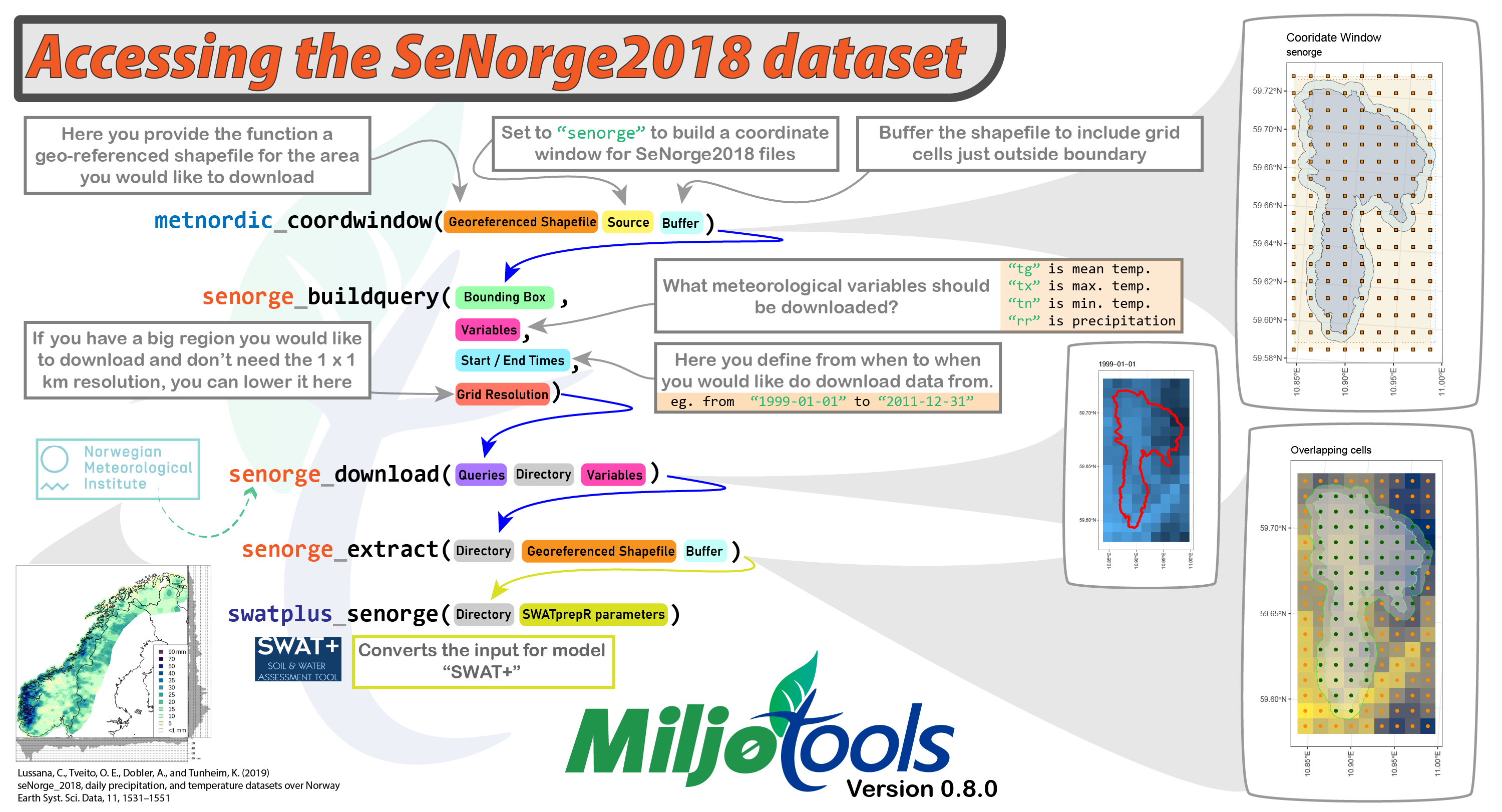
miljotools helps you access this dataset by allowing you to download and apply a subset of the data that interests you. You can do this by:

Determining your coordinate window
Building your download query
Downloading your queries
Extracting data in “.csv” format.
Apply data to models

Flowchart

A useful flowchart on how the miljotools SeNorge functions fit together

Workflow

require(miljotools)
require(sf)
require(mapview)

We need to provide a shapefile (polygon) of our desired area to download. In this example we will download the following publicly available watershed file:

download.file(url = "https://gitlab.nibio.no/moritzshore/example-files/-/raw/main/MetNoReanalysisV3/cs10_basin.zip", destfile = "cs10_basin.zip")
unzip("cs10_basin.zip")
cs10_basin = "cs10_basin/cs10_basin.shp"
example_polygon_geometry <- read_sf(cs10_basin)
map1 <- mapview(example_polygon_geometry, alpha.regions = .3, legend = F)
map1

We can use the same function as for the MET Nordic dataset for SeNorge, we just need to adjust the “project” parameter. We will also buffer the shapefile by 500 m to include grid cells just outside the boundaries.

my_coord_window <- metnordic_coordwindow(
  area_path = example_polygon_geometry,
  area_buffer = 500,
  source = "senorge",
  verbose = TRUE, 
  interactive = FALSE
)

## miljo🌿tools > metnordic_coordwindow  >> getting base file from: SeNorge2018
## miljo🌿tools > metnordic_coordwindow  >> basefile downloaded. 
## miljo🌿tools > metnordic_coordwindow  >> Loading and projecting shapefile... 
## miljo🌿tools > metnordic_coordwindow  >> geometry detected: sfc_POLYGON
## miljo🌿tools > metnordic_coordwindow  >> buffering shapefile:  500 m
## miljo🌿tools > metnordic_coordwindow  >> calculating coordinate window... 
## miljo🌿tools > metnordic_coordwindow  >> coordinate window is: xmin=341 xmax=349 xmin=1388 ymax=1372

Now we can use this coordinate window to build our download queries. At this stage we need to define which variables we should like to download, at which resolution, and for which time period. In this example we are downloading all the variables (tg = mean daily temperature, tn = minimum daily temperature, tx = maximum daily temperature, rr = total daily precipitation), from a random day in 1999 to a random day in 2001. We are doing this at a grid resolution of 1x1.

my_queries <- senorge_buildquery(
  bounding_coords = my_coord_window,
  variables = c("tg", "tn", "tx", "rr"),
  fromdate = "1999-12-30",
  todate = "2000-01-02",
  grid_resolution = 1,
  verbose = TRUE
)

## miljo🌿tools > senorge_buildquery  >> You have a grid of: 8 x 16 (128 cells)
## miljo🌿tools > senorge_buildquery  >> generating urls with a grid resolution of: 1 x 1 km
## miljo🌿tools > senorge_buildquery  >> Returning queries.. (2)

Now that we have our queries, we can download our customized files. We can provide our polygon to double check that the download matches the area we want.

my_download <- senorge_download(
  queries = my_queries,
  directory = "senorge_download",
  variables =  c("tg", "tn", "tx", "rr"),
  polygon = example_polygon_geometry,
  verbose = FALSE
)

Diagnostic plots

With our files downloaded in .nc format, we can convert them to .csv for the grid cells that cover our desired area. (Note: at this stage you can use a different, smaller polgyon if you only want to extract a smaller subset of the available data)

senorge_extract_grid(
  directory = my_download,
  outdir = "senorge_extract_grid",
  area = example_polygon_geometry,
  variables = c("tg", "tn", "tx", "rr"),
  buffer = 500,
  verbose = FALSE,
  map = TRUE
) -> my_extract

Having a look at the results:

list.files(my_extract, pattern = ".csv", full.names = T)[1] %>% readr::read_csv(show_col_types = FALSE)

## # A tibble: 4 × 6
##   vstation date          tg     tn    tx    rr
##      <dbl> <date>     <dbl>  <dbl> <dbl> <dbl>
## 1        1 1999-12-30 -5.59 -10.7  -4.42  0   
## 2        1 1999-12-31 -9.61 -13.5  -8.46  0   
## 3        1 2000-01-01 -9.35  -9.35 -2.75 10.3 
## 4        1 2000-01-02 -5.45  -6.39  3.16  0.47

metadata_path = list.files(my_extract, pattern = ".shp", full.names = T)
metadata_path %>% sf::read_sf() %>% mapview::mapview(label = "vstation", legend = FALSE)

Model Connections

If you are using SWAT+ you can apply the SeNorge data to your setup using the following function:

swatplus_senorge(
  extract_path = my_extract,
  metadata = metadata_path,
  DEM = "../../swat-cs10/model_data/input/elevation/cs10_dem_1m_utm33n.tif",
  aux_data = "../../swat-cs10/model_data/input/met/cs10_weather_data.xlsx",
  epsg_code = 25832,
  write_path = "../../mt-testing/MetNord_MN2/",
  verbose = FALSE
)