Section 2 Building with BuildR
This OPTAIN-style model setup will be created using SWATbuildR
(Schürz Christoph et al. 2022). This allows for a field-scale level of
detail within the SWAT+ model, also known as COCOA …(TBC)
For our model setup, the we need many maps/layers. These include elevation, soil, aquifer, land, and channel, see figure XXX
!['Required vector and rasrer inputs for a SWAT+ model setup with `SWATbuildR`', Figure 2.1 of [@schurz_christoph_swat_2022]](project_data/figures/layers_cococa.jpg)
Figure 2.1: ‘Required vector and rasrer inputs for a SWAT+ model setup with SWATbuildR’, Figure 2.1 of (Schürz Christoph et al. 2022)
We will first set up the BuildR: this will not be needed once the package is released.
# Script version of SWATbuildR -------------------------------------
# Version 1.5.17
# Date: 2023-08-14
# Developer: Christoph Schürz christoph.schuerz@ufz.de
#
# This is a script version of the SWATbuildR workflow that is under
# development. The functional workflow works already as it will be
# implemented in a final R package version.
# Land, channel, reservoir, and point source objects are already
# implemented. Further object types and functional features will be
# implemented over time.
# ------------------------------------------------------------------

# Project path (where output files are saved) ----------------------
project_path <- 'project_data/skuterud_swat/'
project_name <- 'skuterud'

# load functions:
fns <- sapply(list.files('project_data/SWATbuildR/functions', full.names = T), source)
rm(fns)

data_path  <- paste(project_path, project_name, 'data', sep = '/')

## Create data folders
dir.create(paste0(data_path, '/vector'), recursive = T, showWarnings = FALSE)
dir.create(paste0(data_path, '/raster'), recursive = T, showWarnings = FALSE)

## Create data folders
dir.create(paste0(data_path, '/vector'), recursive = T, showWarnings = FALSE)
dir.create(paste0(data_path, '/raster'), recursive = T, showWarnings = FALSE)

## Check if the installed R version is greater than the required one
check_r_version('4.2.1')

## Install and load R packages
install_load(crayon_1.5.1, dplyr_1.0.10, forcats_0.5.1, ggplot2_3.3.6,
             lubridate_1.8.0, purrr_1.0.0, readr_2.1.2, readxl_1.4.0,
             stringr_1.4.0, tibble_3.1.8, tidyr_1.2.0, vroom_1.5.7)
install_load(sf_1.0-8, sfheaders_0.4.0, lwgeom_0.2-8, terra_1.7-3,
             whitebox_2.1.5, units_0.8-0)
install_load(DBI_1.1.3, RSQLite_2.2.15)

# wbt_exe <- list.files(path = find.package("whitebox"),
#                       pattern = 'whitebox_tools.exe',
#                       recursive = TRUE, full.names = TRUE)
# wbt_init(exe_path = wbt_exe)
Our first step for this setup is to process the digital elevation model (DEM).
Required packages for this section:
2.1 DEM
The DEM is necessary for a variety of things within our model setup, such as the watershed, stream network, and object connectivities.
The DEM we will use is sourced from hoydedata.no and has full coverage of Norway at 1m resolution. It is important that we use a high resolution DEM as our flow routes and connectivity calculations depend on elements such as elevated road networks:
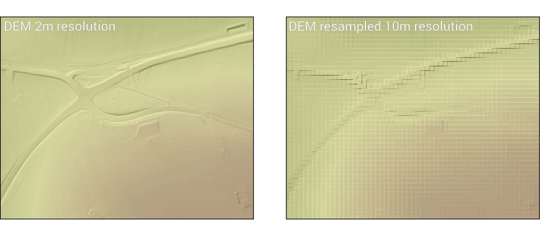
Figure 2.2: Schürz et al. (2022)
The tile with coverage of our catchment “Skuterud” is dtm1_33_124_113.
This raster map is in .tif format. We can read in a (low resolution
preview) map of this file using mapview and terra.
We know approximately where our catchment will be:
approx <- read_sf("project_data/input/DEM/reference/skuterud_general_area.shp")
mapview(approx, map.types = "Esri.WorldImagery")
We can crop our large DEM file to this estimation, which will dramatically reduce computation times.
DEM_crop <- terra::crop(x = DEM, y = approx)
terra::writeRaster(x = DEM_crop, filename = "project_data/input/DEM/skuterud_DEM.tif")
2.1.1 Watershed
To start, we need to delineate our catchment boundaries, which we will do with the digital elevation map.
Processing of this map will be done with the help of WhiteBoxTools (ref).
First we breach depressions.
Question, is fill = TRUE ok here? Are there any other parameters that
should be adjusted?
wbt_breach_depressions_least_cost(
  dem = "project_data/input/DEM/skuterud_DEM.tif",
  output = "project_data/input/DEM/wbt_intermediates/breached_depressions.tif",
  dist = 5, # Maximum search distance for breach paths in cells.
  fill = TRUE # Optional flag indicating whether to fill any remaining unbreached depressions.
  )
Time to calculate our flow accumulation using the D8 algorithm.
wbt_d8_flow_accumulation(
  input = "project_data/input/DEM/wbt_intermediates/breached_depressions.tif",
  output = "project_data/input/DEM/wbt_intermediates/flow_accumulation.tif")
And the D8 pointer:
wbt_d8_pointer(
  dem = "project_data/input/DEM/wbt_intermediates/breached_depressions.tif",
  output = "project_data/input/DEM/wbt_intermediates/d8_pointer.tif"
  )
Where is our catchment outlet? It is located here:
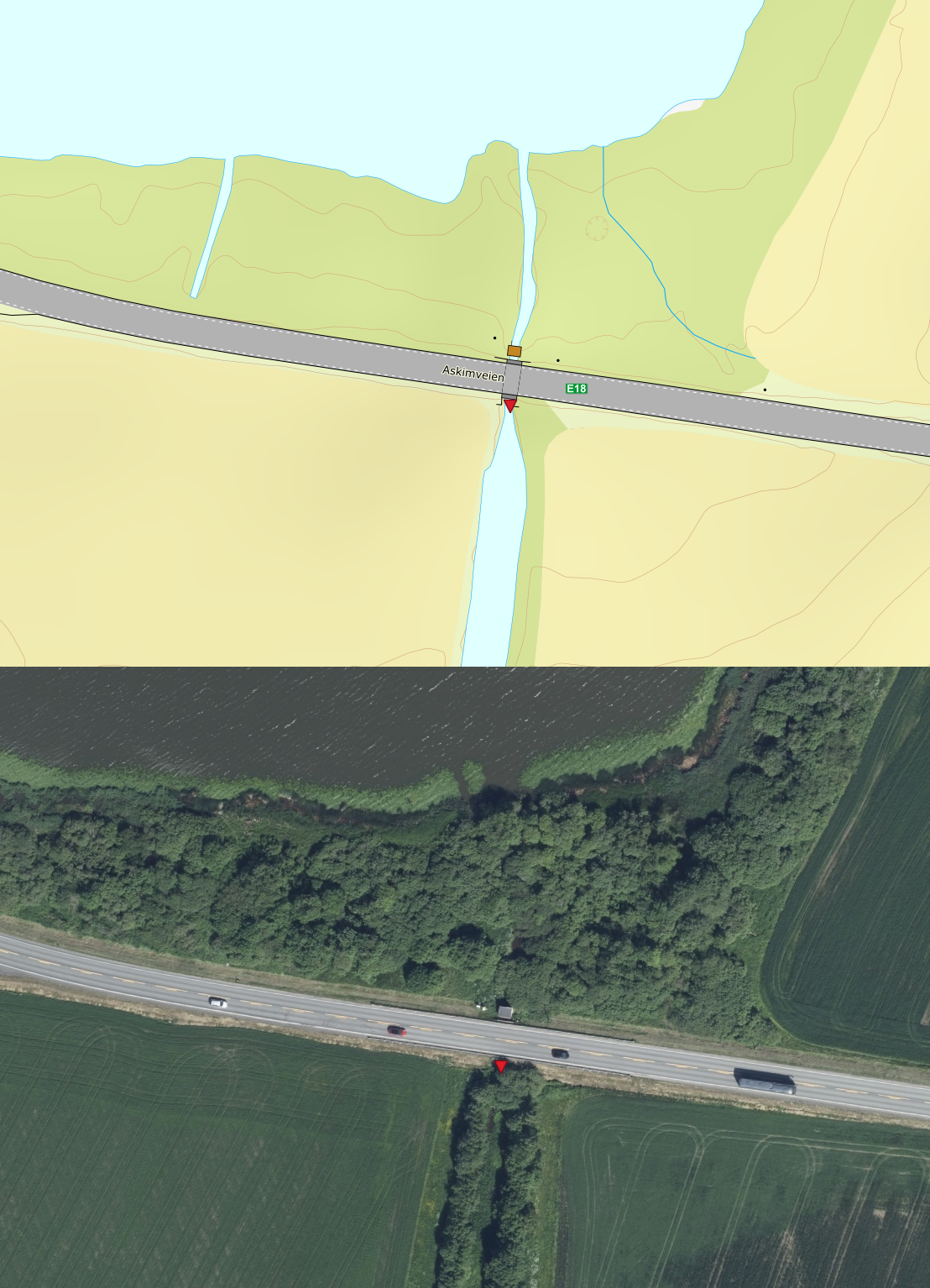
Figure 2.3: Skuterud Outlet
The measuring station itself is actually behind the road, where a tunnel leads directly to the instruments, however to get an accurate basin from the DEM, this allocation is most correct, as water north of the road does not make it into the station.
outlet <- "project_data/input/DEM/point/skuterud_outlet.shp"
outlet_point <- sf::read_sf(outlet)
outlet_map <- mapview::mapview(outlet_point, map.types = "Esri.WorldImagery")
outlet_map
Now that we have our outlet point, we need to snap it to our stream network. For that we need a stream network.
wbt_extract_streams(
  flow_accum = "project_data/input/DEM/wbt_intermediates/flow_accumulation.tif",
  output ="project_data/input/DEM/wbt_intermediates/raster_streams.tif",
  threshold = 10000)
Lets have a look:
stream_rast <- terra::rast("project_data/input/DEM/wbt_intermediates/raster_streams.tif")
plot(stream_rast)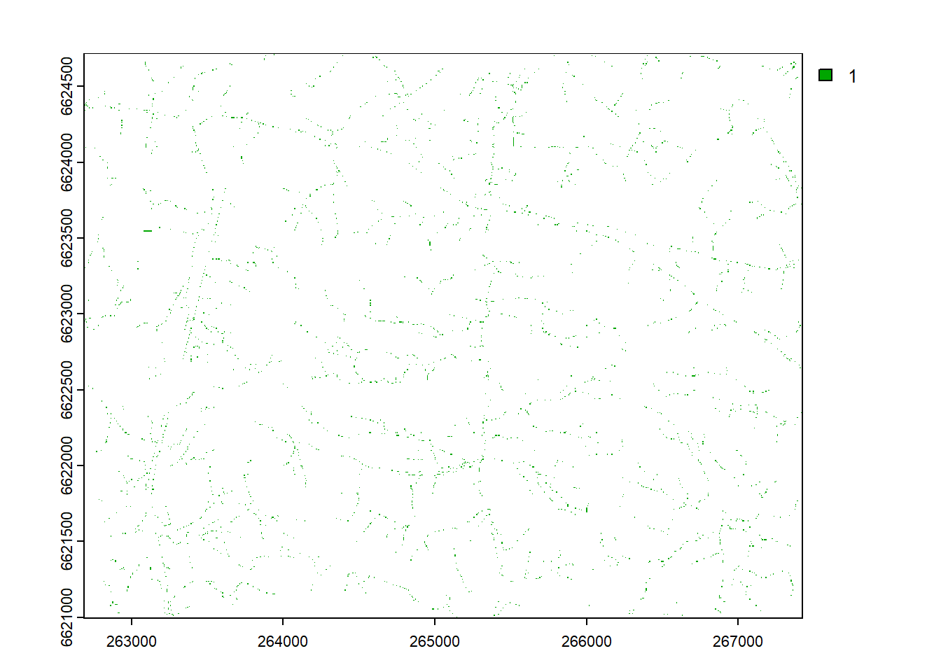
Little hard to see, lets zoom in on the outlet (we got these coords from QGIS)
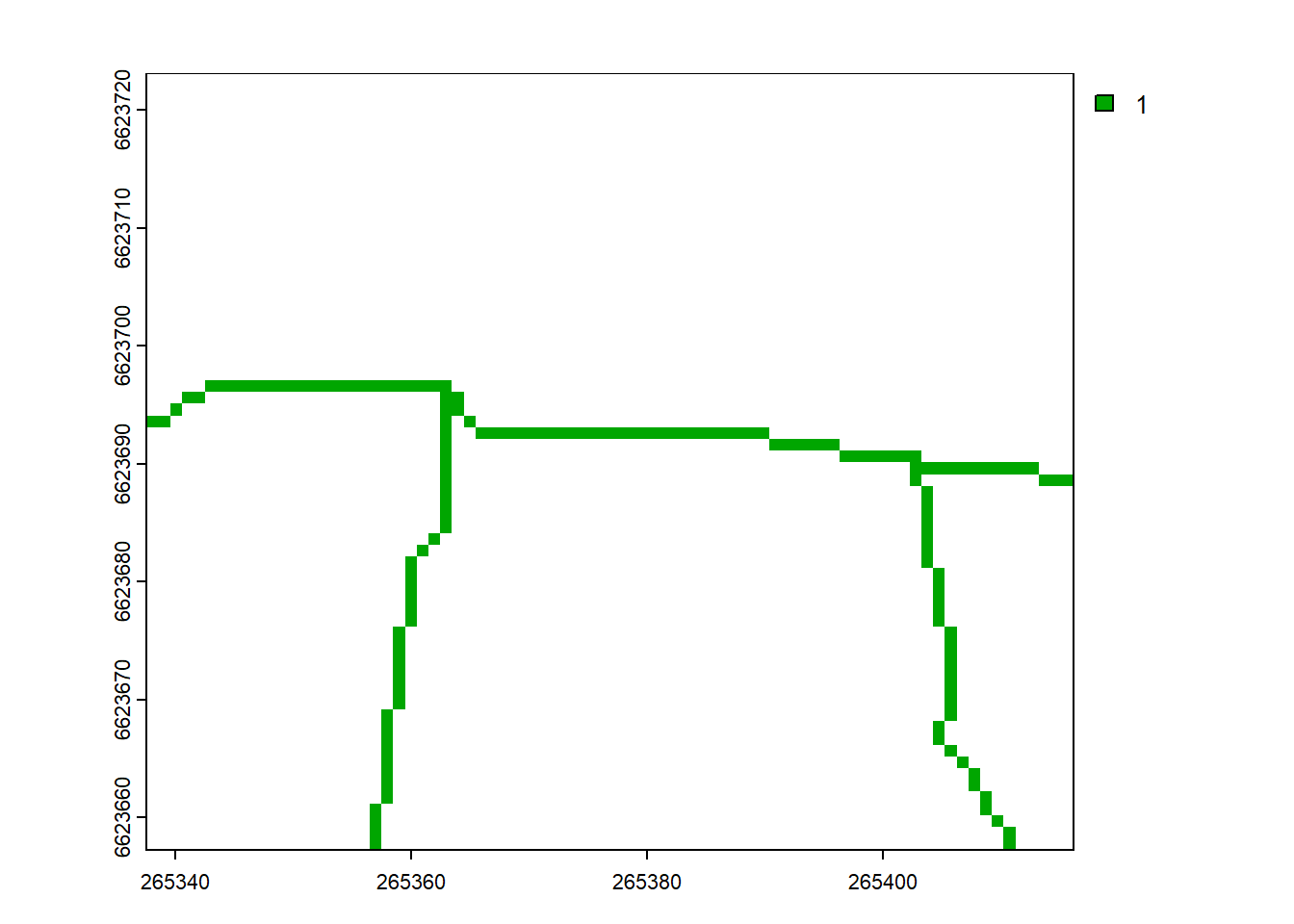
Hmm… This does not look good. The streams flow to the left and cross into the lake somewhere in the east. This does not match reality. Why is this occurring? Its probably because of the elevated road which the stream passes under. This is a common issue and you can read more about it here.
But lets get to fixing it by burning in our known stream network from NVE’s map service NEVINA, specifically ELVIS.
nve_stream_network <- sf::read_sf("project_data/input/DEM/line/stream_network/NVEData/Elv/Elv_Elvenett.shp") %>% select(geometry, elvID)
nve_crop <- st_crop(nve_stream_network, st_buffer(approx, 10000))
## Warning: attribute variables are assumed to be spatially constant throughout
## all geometriesLooks good. We shall save it
The NVE stream network is not quite detailed enough to show all the important streams. Therefore it was extended slightly. This step is important because the underground stream passages through the road network will determine the watershed later on.
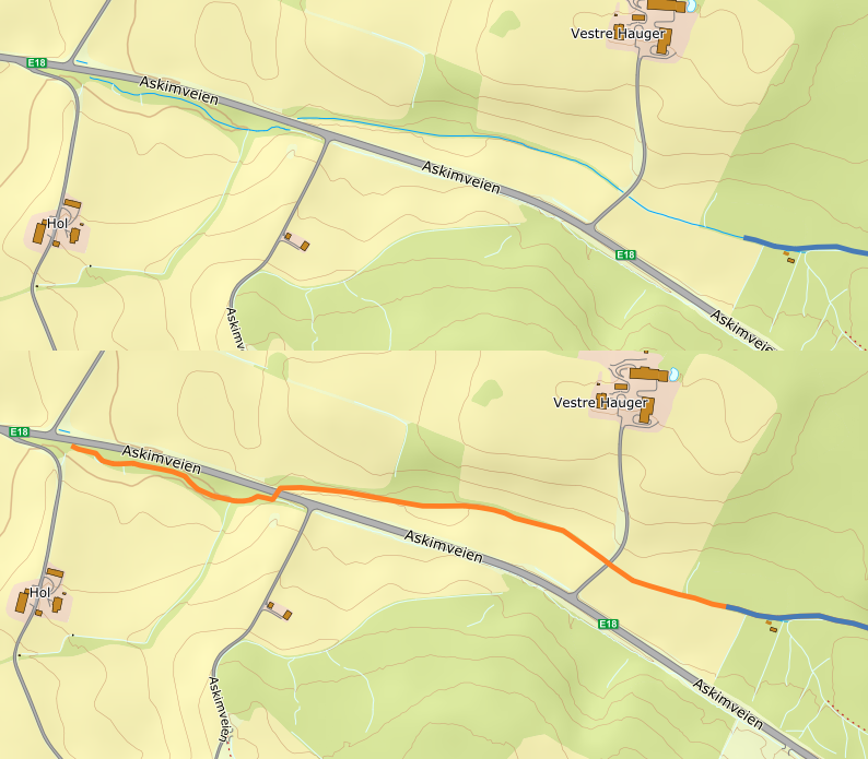
Figure 2.4: Extended stream over road.
Burning in the stream network to deal with this r:
whitebox::wbt_fill_burn(
  dem = "project_data/input/DEM/skuterud_DEM.tif",
  streams = "project_data/input/DEM/line/stream_network/skuterud_testbed.shp",
  output =  "project_data/input/DEM/wbt_intermediates/fill_burn.tif")
Now repeating the whole process:
wbt_breach_depressions_least_cost(
  dem = "project_data/input/DEM/wbt_intermediates/fill_burn.tif",
  output = "project_data/input/DEM/wbt_intermediates/breached_depressions_burn.tif",
  dist = 5, # Maximum search distance for breach paths in cells.
  fill = TRUE # Optional flag indicating whether to fill any remaining unbreached depressions.
  )
wbt_d8_flow_accumulation(
  input = "project_data/input/DEM/wbt_intermediates/breached_depressions_burn.tif",
  output = "project_data/input/DEM/wbt_intermediates/flow_accumulation_burn.tif")
wbt_d8_pointer(
  dem = "project_data/input/DEM/wbt_intermediates/breached_depressions_burn.tif",
  output = "project_data/input/DEM/wbt_intermediates/d8_pointer_burn.tif"
  )
wbt_extract_streams(
  flow_accum = "project_data/input/DEM/wbt_intermediates/flow_accumulation_burn.tif",
  output ="project_data/input/DEM/wbt_intermediates/raster_streams_burn.tif",
  threshold = 10000)

stream_rast <- terra::rast("project_data/input/DEM/wbt_intermediates/raster_streams_burn.tif")
plot(stream_rast, xlim = c(265337.49,265416.12), ylim = c(6623657.26, 6623723.11))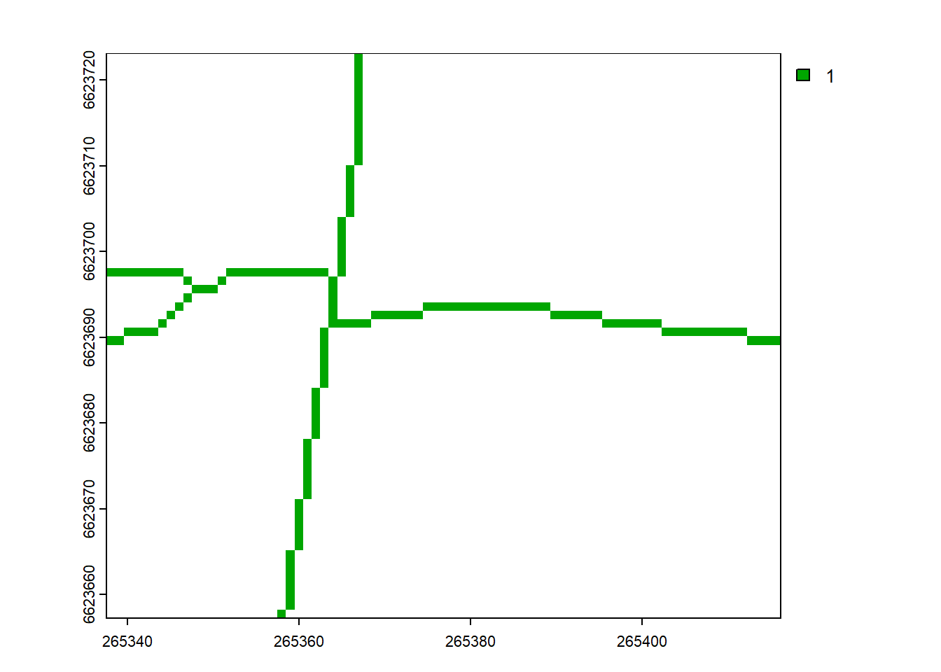
Yes! Looks good. Now:
Sticking the point on the stream:
wbt_jenson_snap_pour_points(
  pour_pts = "project_data/input/DEM/point/skuterud_outlet.shp",
  streams = "project_data/input/DEM/wbt_intermediates/raster_streams_burn.tif",
  output = "project_data/input/DEM/point/outlet_snapped.shp",
  snap_dist = 5) #careful with this! Know the units of your data
Lets have a look at that snap shall we?
snap_outlet <- sf::read_sf("project_data/input/DEM/point/outlet_snapped.shp")
snap_mapped <- mapview::mapview(snap_outlet, map.types = "Esri.WorldImagery")
snap_buffer <- sf::st_buffer(snap_outlet, 100)
stream_rast <- terra::rast("project_data/input/DEM/wbt_intermediates/raster_streams_burn.tif")

streams_cropped <- terra::crop(stream_rast, snap_buffer)
streams_map <- mapview::mapview(streams_cropped, map.types = "Esri.WorldImagery")
streams_map+snap_mapped
Looking good, looking great. Moving on:
Its the big moment, time to delineate our watershed:
wbt_watershed(
  d8_pntr = "project_data/input/DEM/wbt_intermediates/d8_pointer_burn.tif",
  pour_pts = "project_data/input/DEM/point/outlet_snapped.shp",
  output = "project_data/input/DEM/wbt_intermediates/skuterud_basin_1m.tif"
  )
Take it out of the oven, and have a look:
WS <- terra::rast("project_data/input/DEM/wbt_intermediates/skuterud_basin_1m.tif")
# convert to polygon
wsshape <- stars::st_as_stars(WS) %>% sf::st_as_sf(merge = T)
## Warning in CPL_read_gdal(as.character(x), as.character(options),
## as.character(driver), : GDAL Message 1: The definition of geographic CRS
## EPSG:4258 got from GeoTIFF keys is not the same as the one from the EPSG
## registry, which may cause issues during reprojection operations. Set
## GTIFF_SRS_SOURCE configuration option to EPSG to use official parameters
## (overriding the ones from GeoTIFF keys), or to GEOKEYS to use custom values
## from GeoTIFF keys and drop the EPSG code.## Warning in CPL_polygonize(file, mask_name, "GTiff", "Memory", "foo", options, :
## GDAL Message 1: The definition of geographic CRS EPSG:4258 got from GeoTIFF
## keys is not the same as the one from the EPSG registry, which may cause issues
## during reprojection operations. Set GTIFF_SRS_SOURCE configuration option to
## EPSG to use official parameters (overriding the ones from GeoTIFF keys), or to
## GEOKEYS to use custom values from GeoTIFF keys and drop the EPSG code.## Warning in abbreviate_shapefile_names(obj): Field names abbreviated for ESRI
## Shapefile driver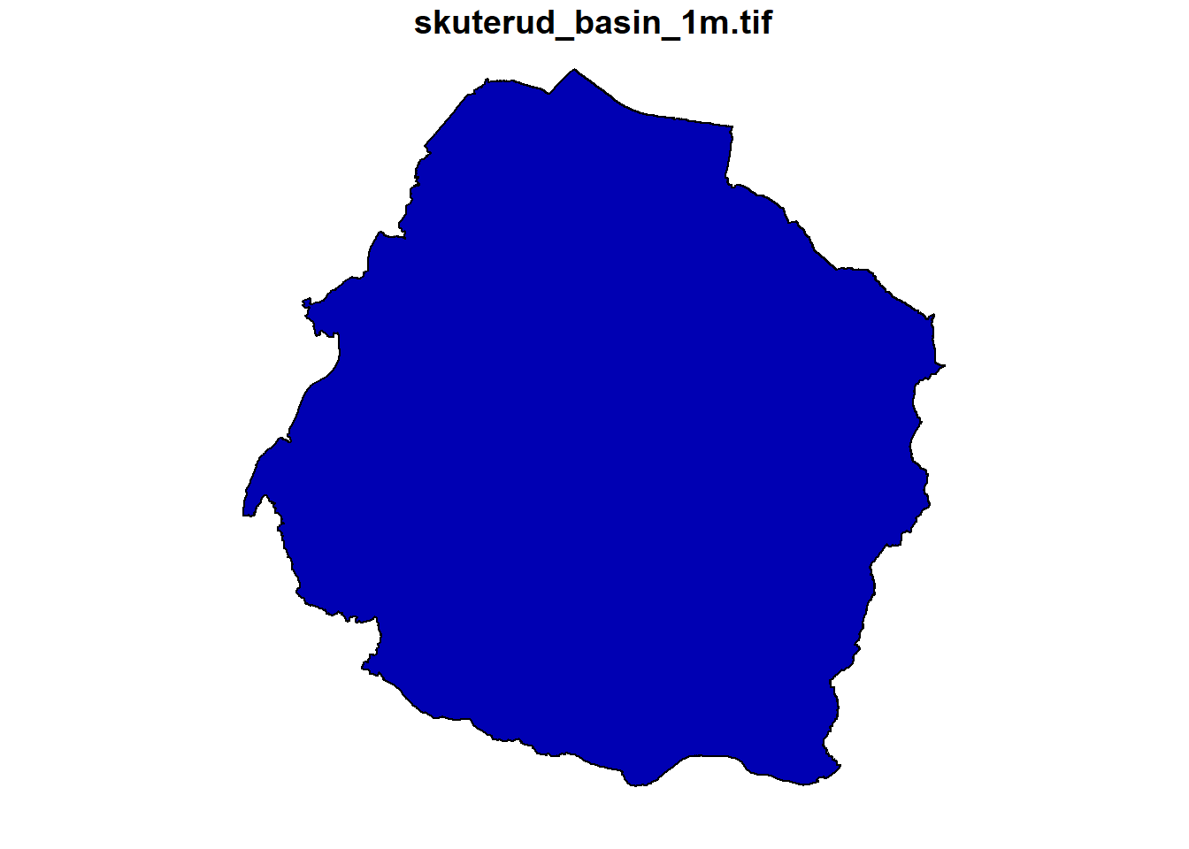
That looks good. lets compare it to some literature on Skuterud, from (Bechmann and Deelstra 2006):
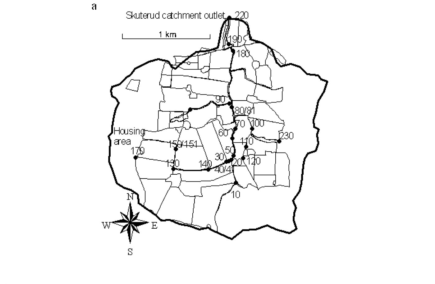
Figure 2.5: Marianne E. Bechmann & Johannes Deelstra (2006)
Quite a big difference in the northwest. The reason for this is an underground channel that feeds water from this field directly into the lake, bypassing the monitoring station. Only during heavy loads will water spill over into the station (personal communication).
This is the drainage system, as seen from Google street view:
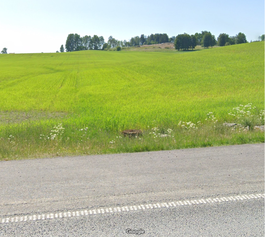
Figure 2.6: Drainage system, Google streetview
This means we need to adapt our stream network. This has been done in QGIS like so:
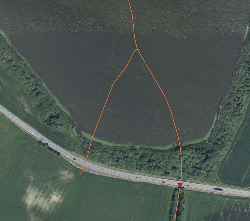
Figure 2.7: Added stream for drainage tunnel
We need to re-do the whole process again:
whitebox::wbt_fill_burn(
  dem = "project_data/input/DEM/skuterud_DEM.tif",
  streams = "project_data/input/DEM/line/stream_network/skuterud_drained.shp",
  output =  "project_data/input/DEM/wbt_intermediates/fill_drained.tif")

wbt_breach_depressions_least_cost(
  dem = "project_data/input/DEM/wbt_intermediates/fill_drained.tif",
  output = "project_data/input/DEM/wbt_intermediates/breached_depressions_drained.tif", dist = 5, fill = TRUE
)

wbt_d8_flow_accumulation(
  input = "project_data/input/DEM/wbt_intermediates/breached_depressions_drained.tif",
  output = "project_data/input/DEM/wbt_intermediates/flow_accumulation_drained.tif")

wbt_d8_pointer(
  dem = "project_data/input/DEM/wbt_intermediates/breached_depressions_drained.tif",
  output = "project_data/input/DEM/wbt_intermediates/d8_pointer_drained.tif"
)

wbt_extract_streams(
  flow_accum = "project_data/input/DEM/wbt_intermediates/flow_accumulation_drained.tif",
  output ="project_data/input/DEM/wbt_intermediates/raster_streams_drained.tif",
  threshold = 10000)

wbt_jenson_snap_pour_points(
  pour_pts = "project_data/input/DEM/point/skuterud_outlet.shp",
  streams = "project_data/input/DEM/wbt_intermediates/raster_streams_drained.tif",
  output = "project_data/input/DEM/point/outlet_snapped.shp",
  snap_dist = 5)

wbt_watershed(
  d8_pntr = "project_data/input/DEM/wbt_intermediates/d8_pointer_drained.tif",
  pour_pts = "project_data/input/DEM/point/outlet_snapped.shp",
  output = "project_data/input/DEM/wbt_intermediates/skuterud_basin_1m.tif"
)

WS <- terra::rast("project_data/input/DEM/wbt_intermediates/skuterud_basin_1m.tif")
wsshape2 <- stars::st_as_stars(WS) %>% sf::st_as_sf(merge = T)
## Warning in CPL_read_gdal(as.character(x), as.character(options),
## as.character(driver), : GDAL Message 1: The definition of geographic CRS
## EPSG:4258 got from GeoTIFF keys is not the same as the one from the EPSG
## registry, which may cause issues during reprojection operations. Set
## GTIFF_SRS_SOURCE configuration option to EPSG to use official parameters
## (overriding the ones from GeoTIFF keys), or to GEOKEYS to use custom values
## from GeoTIFF keys and drop the EPSG code.## Warning in CPL_polygonize(file, mask_name, "GTiff", "Memory", "foo", options, :
## GDAL Message 1: The definition of geographic CRS EPSG:4258 got from GeoTIFF
## keys is not the same as the one from the EPSG registry, which may cause issues
## during reprojection operations. Set GTIFF_SRS_SOURCE configuration option to
## EPSG to use official parameters (overriding the ones from GeoTIFF keys), or to
## GEOKEYS to use custom values from GeoTIFF keys and drop the EPSG code.## Warning in abbreviate_shapefile_names(obj): Field names abbreviated for ESRI
## Shapefile driverLooks good. A comparison:
mapview(wsshape, map.types = "Esri.WorldImagery") + mapview(wsshape2, col.region = "orange", map.types = "Esri.WorldImagery")2.1.1.1 BuildR Implementation
Now that we have our watershed ready, we can implement it into the BuildR
bound_path = "project_data/input/DEM/skuterud_basin_1m_drained.shp"
bound <- read_sf(bound_path) %>% select()
set_proj_crs(bound, data_path)
check_polygon_topology(layer = bound, data_path =  data_path, label = 'basin',
                       n_feat = 1, checks = c(F,T,T,T,F,F,F,F))
## Running topological checks and modifications for the basin layer:
##
## Analyzing basin layer for specific number of features...
## ✔ Number of features correct.
## Analyzing basin layer for MULTIPOLYGON features...
## ✔ No MULTIPOLYGON features identified.
## Analyzing basin layer for invalid features...
## ✔ No invalid features identified.
##
##
## ✔ All checks successful! Saving checked basin layer.An unnumbered section
BuildR progress:
# Read and prepare input data --------------------------------------
## Basin boundary
# done


## Load and check the soil raster layer
soil <- rast(soil_layer_path) %>%
  check_project_crs(layer = ., data_path =  data_path, proj_layer = project_layer,
                    label = 'soil', type = 'raster')
check_raster_coverage(rst = soil, vct_layer = 'hru', data_path = data_path,
                      label = 'soil', cov_frc = 0.75)
## Project the soil layer to the grid and crs of the DEM
save_soil_raster(soil, data_path)

## Prepare table with aggregated elevation, slope, soil for HRU units.
aggregate_hru_dem_soil(data_path)

## Read and prepare the soil input tables and a soil/hru id table and write
## them into data_path/tables.sqlite
build_soil_data(soil_lookup_path, soil_data_path, data_path)

# Calculate land unit connectivity ---------------------------------
## Prepare raster layers based on the DEM and the surface channel objects
## that will be used in the calculation of the land object connectivity.
prepare_terrain_land(data_path)

## Calculate the land object connectivity. The connection of each land
## object to neighboring land and water objects is calculated based on
## the flow accumulation and the D8 flow pointer along the object edge
calculate_land_connectivity(data_path)

## Eliminate land object connections with small flow fractions.
## For each land object the flow fractions are compared to connection with
## the largest flow fraction of that land object. Connections are removed
## if their fraction is smaller than 'frc_thres' relative to the largest one.

## The remaining land object connections are analyzed for infinite loop
## routing. For each land unit the connections are propagated and checked
## if the end up again in the same unit.
reduce_land_connections(data_path, frc_thres) %>%
  check_infinite_loops(., data_path, 'Land')

## If infinite loops were identified this routine tries to resolve the
## issues by selectively removing connections between land units in order
## to get rid of all infinite loops.
resolve_loop_issues(data_path)

# Calculate channel/reservoir connectivity -------------------------
## Calculate the water object connectivity. The function returns the cha
## and res con_out tables in SWAT+ database format and writes them into
## data_path/tables.sqlite
build_water_object_connectivity(data_path)

## Check the water objects for infinite loops. From the cha_res_con_out
## tables id_from/id_to links are generated and checked for infinite
## loop routing.
prepare_water_links(data_path) %>%
  check_infinite_loops(., data_path, 'Water', Inf)

## Calculate terrain properties such as elevation, slope, catchment area,
## channel width/depth for channel and reservoir objects and write them into
## data_path/tables.sqlite
prepare_terrain_water(data_path)

# Generate land object SWAT+ input tables --------------------------
## Build the landuse.lum and a landuse/hru id table and write them into
## data_path/tables.sqlite
build_landuse(data_path)

## Build the HRU SWAT+ input files and write them into data_path/tables.sqlite
build_hru_input(data_path)

## Add wetlands to the HRUs and build the wetland input files and write them
## into data_path/tables.sqlite
add_wetlands(data_path, wetland_landuse)

# Generate water object SWAT+ input tables -------------------------
## Build the SWAT+ cha input files and write them into data_path/tables.sqlite
build_cha_input(data_path)

## Build the SWAT+ res input files and write them into data_path/tables.sqlite
build_res_input(data_path)

## Build SWAT+ routing unit con_out based on 'land_connect_fraction'.
build_rout_con_out(data_path)

## Build the SWAT+ rout_unit input files and write them into
## data_path/tables.sqlite
build_rout_input(data_path)

## Build the SWAT+ LSU input files and write them into data_path/tables.sqlite
build_ls_unit_input(data_path)

# Build aquifer input ----------------------------------------------
## Build the SWAT+ aquifer input files for a single aquifer for the
## entire catchment. The connectivity to the channels with geomorphic
## flow must be added after writing the txt input files.
## This is not implemented in the script yet.
build_single_aquifer_files(data_path)

# Add point source inputs ------------------------------------------
## Add point source inputs. The point source locations are provided
## with a point vector layer in the path 'point_path'. Point source
## records can automatically be added from files in the same folder
## as the point source location layer. To be identified as point
## source data the files must be named as <name>_<interval>.csv,
## where <name> must be the name of a point int the vector layer
## and <interval> must be one of 'const', 'yr', 'mon', or 'day'
## depending on the time intervals in the input data.
add_point_sources(point_path, data_path, max_point_dist)

# Create SWAT+ sqlite database -------------------------------------
## Write the SWAT+Editor project database. The database will be located
## the 'project_path'. After writing the database it can be opened and
## edited with the SWAT+Editor.
create_swatplus_database(project_path, project_name)

# -------------------------------------------------------------------------
# Switch to SWAT+Editor for further model parametrization
# and continue with the step below after writing
# the SWAT+ projects' text input files
# -------------------------------------------------------------------------

# Link aquifers and channels with geomorphic flow -------------------------
# A SWATbuildR model setup only has one single aquifer (in its current
# version). This aquifer is linked with all channels through a channel-
# aquifer-link file (aqu_cha.lin) in order to maintain recharge from the
# aquifer into the channels using the geomorphic flow option of SWAT+
# The required input file cannot be written with the SWAT+Editor.
# Therefore it has to be generated in a step after writing the
# model text input files with the SWAT+Editor.
link_aquifer_channels(txt_path)