Section 3 Land Use Map
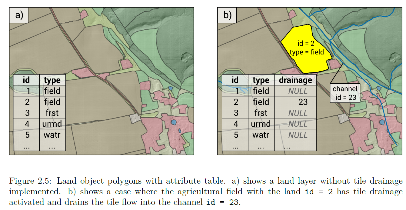
In this section we will construct the land use map.. The final result will resemble figure 2.5 from (Schürz Christoph et al. 2022):
3.1 AR5 Base map
As a basis for our land use we will use the AR5 map from NIBIO. A lower resolution version of this map can be downloaded from Kart8, and then high resolution map can be viewed in Kilden.
The map has been pre-clipped to our research area to save on computational and data costs.
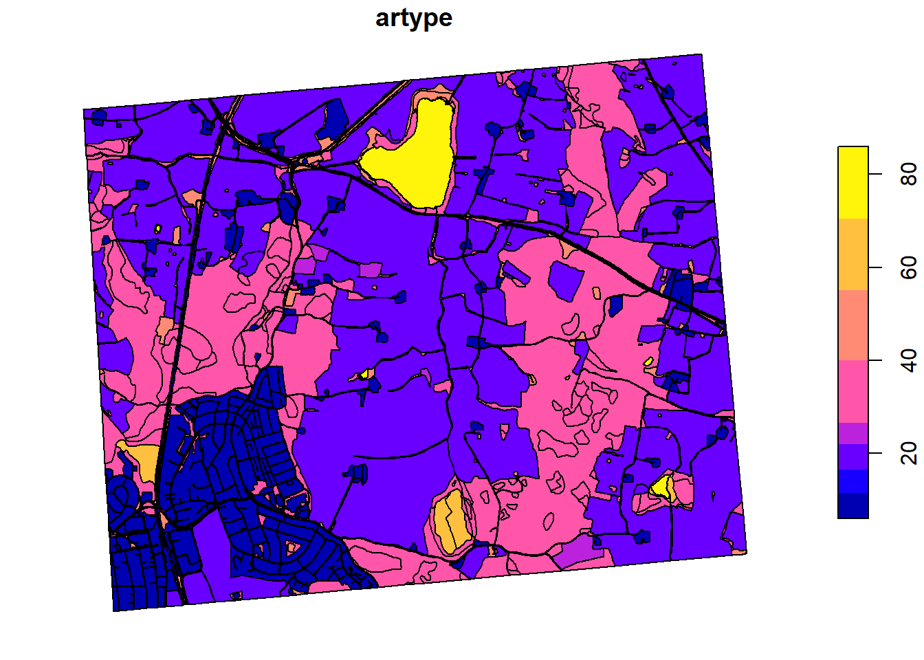
We are only interested in the artype column, so we will extract the
geometry and the artype
And we will re class the legend items into a legend SWATbuildR can
understand.
ar5_sel$type <- NA
ar5_sel$type[which(ar5_sel$artype==11)] = "urml"
ar5_sel$type[which(ar5_sel$artype==12)] = "utrn"
ar5_sel$type[which(ar5_sel$artype==21)] = "agri"
ar5_sel$type[which(ar5_sel$artype==22)] = "past"
ar5_sel$type[which(ar5_sel$artype==23)] = "past"
ar5_sel$type[which(ar5_sel$artype==30)] = "frst"
ar5_sel$type[which(ar5_sel$artype==50)] = "rngb"
ar5_sel$type[which(ar5_sel$artype==60)] = "wetf"
ar5_sel$type[which(ar5_sel$artype==81)] = "watr"
plot(ar5_sel["type"])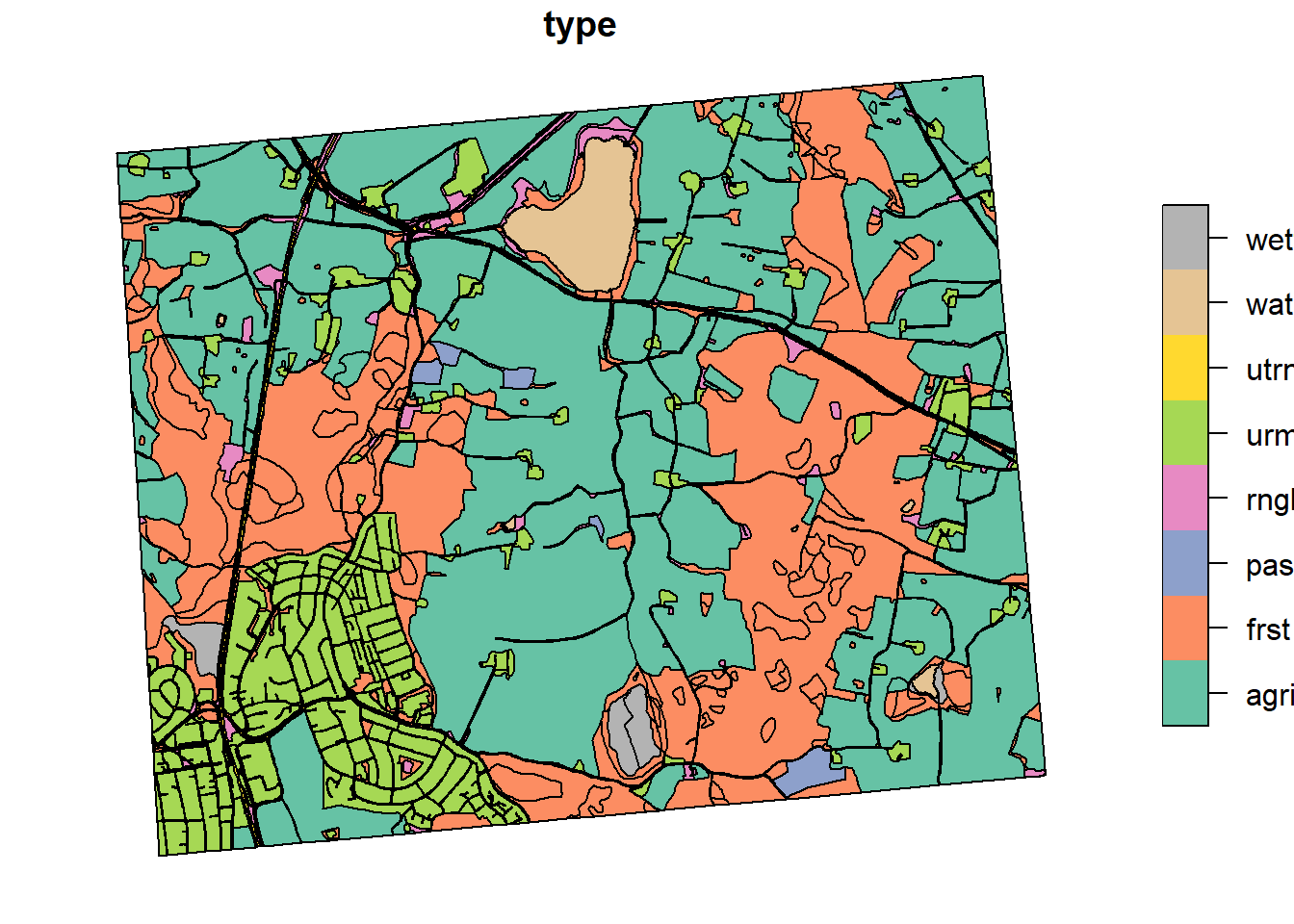
Time to save this file
To minimize computation time, we need to minimize the amount of polygons in this layer.
## [1] 1161Taking a closer look at the map:
WS <- mapview(read_sf("project_data/input/DEM/skuterud_basin_1m_drained.shp"), alpha.region = 0, lwd = 3)
LU <- mapview(ar5_sel, zcol = "type", alpha.region = 0.1)
WS+LUThere is much to remove and simplify, but before we do that, we should make sure we reach maximum “complexity” in our map. This is because if we simplify now, and then later burn in more polygons, our efforts will be wasted / inefficient. The first thing we need to add is the farm fields themselves.
3.2 Farm Fields
As this setup is aiming to represent the field scale, we need to add the fields into our “landscape”. The catchment we have chosen is a “JOVA” catchment which monitors all sorts of things going on in the catchment, including what operations are conducted on all the fields. You can read about JOVA here. The delineation of th fields was provided to us by the JOVA team. Let’s take a look at the map:
jova_skut_fields <- read_sf("project_data/input/LU/agriculture/skifter_sku2.shp")
jova_map <- mapview(jova_skut_fields, alpha.region = .1, col.region = "orange")
jova_mapIt looks good, however, comparing it to the agricultural land from our basemap “AR5” reveals a problem:
Quite a bit of overlap. There (to my best knowledge) is no way of fixing this issue other than manual correction, which will be done in QGIS and documented here. The goal is a final map compatible with AR5 data.
To start, we will extract just the agricultural fields, and save them to a file to be modified:
farm_map <- ar5_sel %>% filter(type == "agri") %>% write_sf("project_data/input/LU/basemap/AR5_agri.shp")Here is the result of the manual QGIS work:
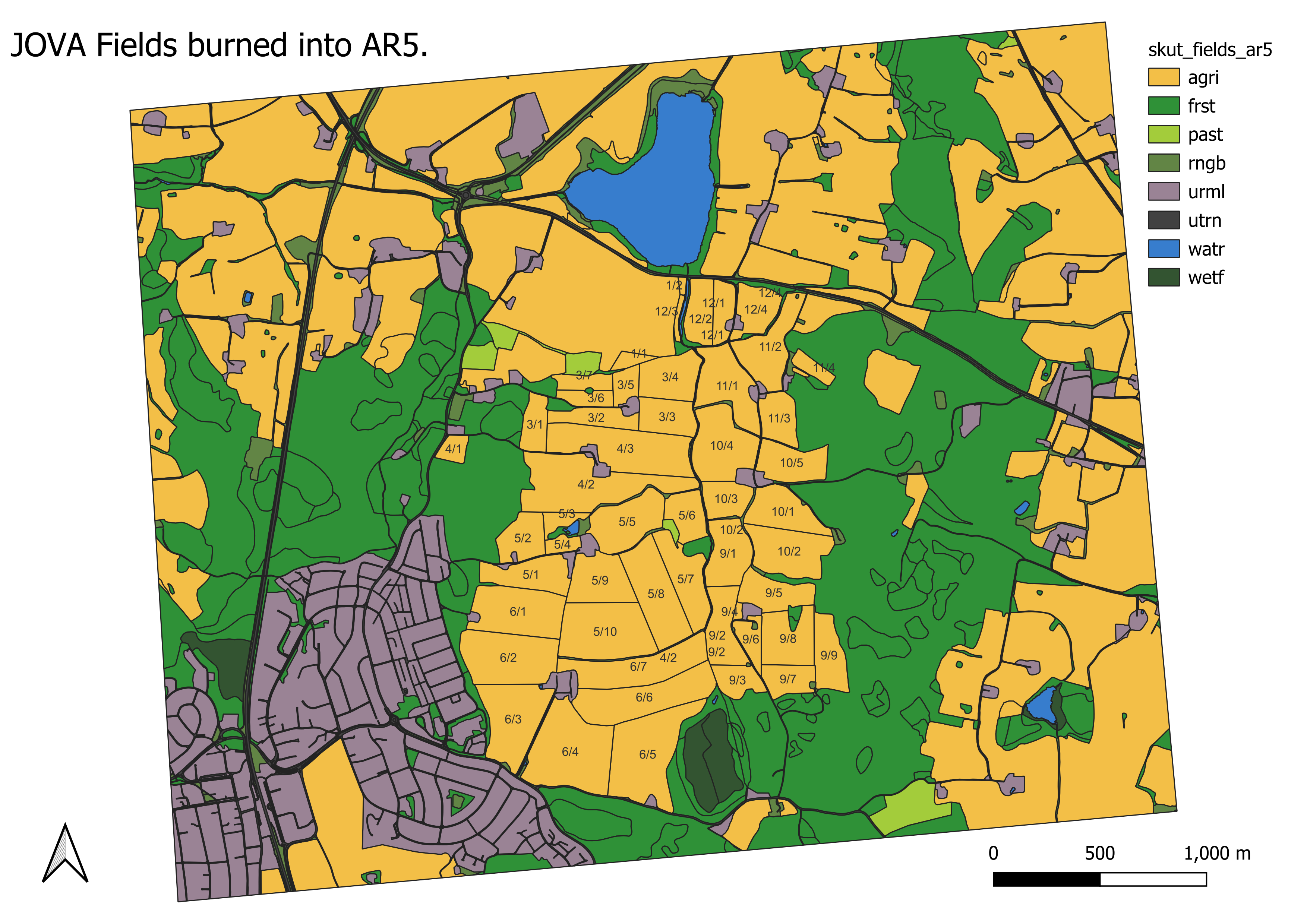
Figure 3.1: JOVA fields burned into AR5, work performed manually with QGIS
We can load this map in now
3.3 Dissolving superfluous polygons
3.3.1 Removing Stream Polygons
Our model setup, following the OPTAIN style setup, does not resolve
water channels (streams) as polygons, instead they are encoded in “line”
geometries. Our AR5 base map treats channels as polygons, therefore we
need to remove them. This was done by replacing the watr type with
either the neighboring rngb or frst.
plot(lu_v2['type'], xlim = c(603080.78,603192.64), ylim = c(6617292.19, 6617120.26))
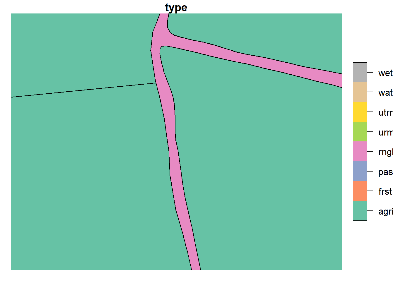
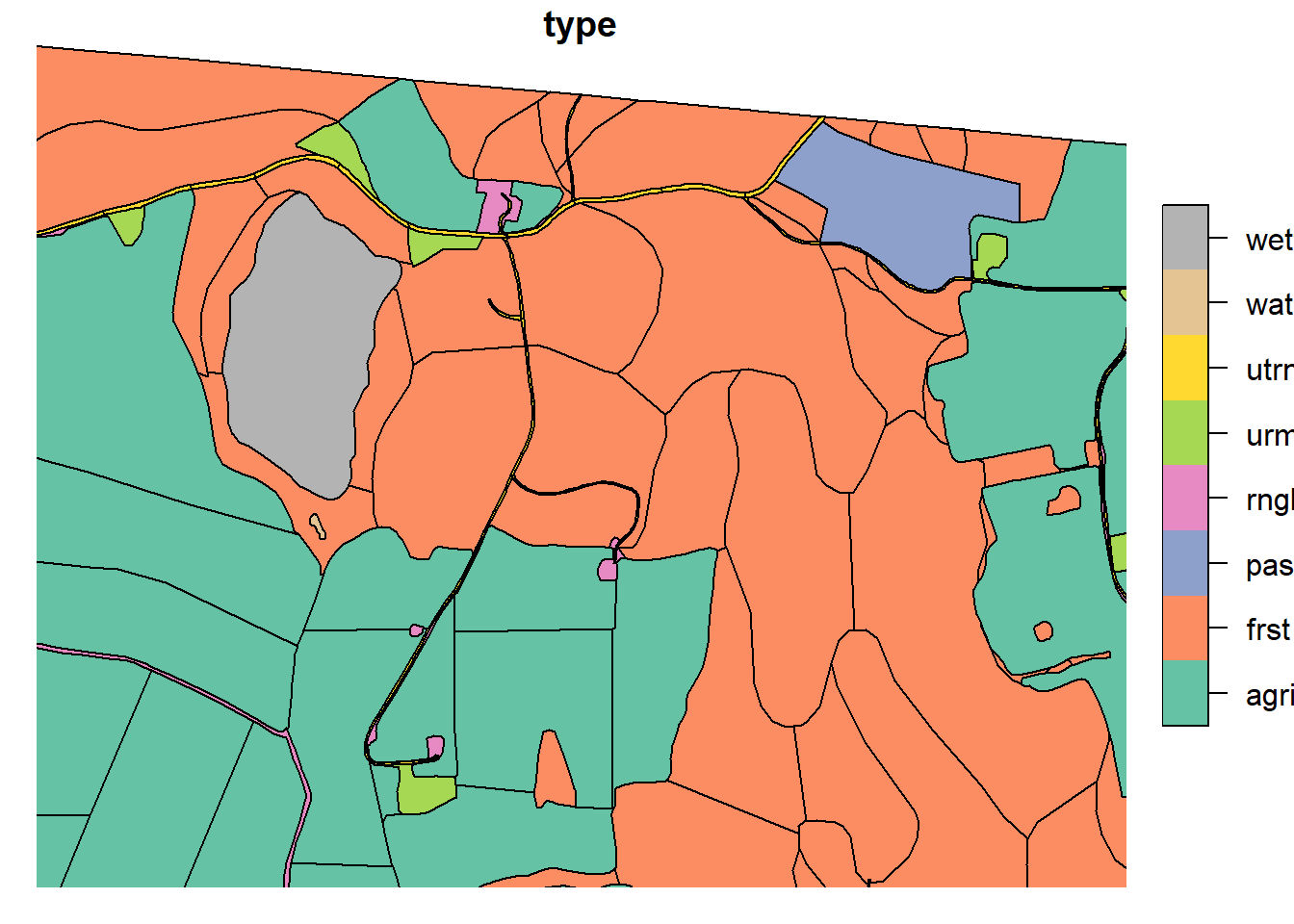
lu_simple <- read_sf("project_data/input/LU/simplification/lu_simple_2.shp")
plot(lu_simple['type'], xlim = c(603080.78,603192.64), ylim = c(6617292.19, 6617120.26)) 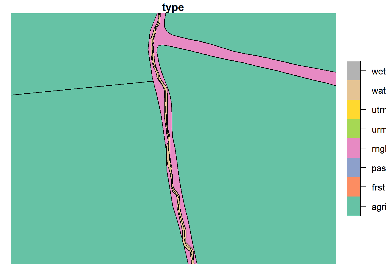
3.3.2 Merging urban and road
In the urbanized part of our catchment (Ås), the road and urban polygons
make up a complex network. As this model setup does not seek to resolve
complex urban landscapes, we can safely reduce the complexity of “urban”
urml and “road” utrn land uses in our map.
par(mar = c(4, 4, .1, .1))
plot(lu_v2['type'], xlim = c(601388.5,602807.8), ylim = c(6616711.7, 6615482.1))
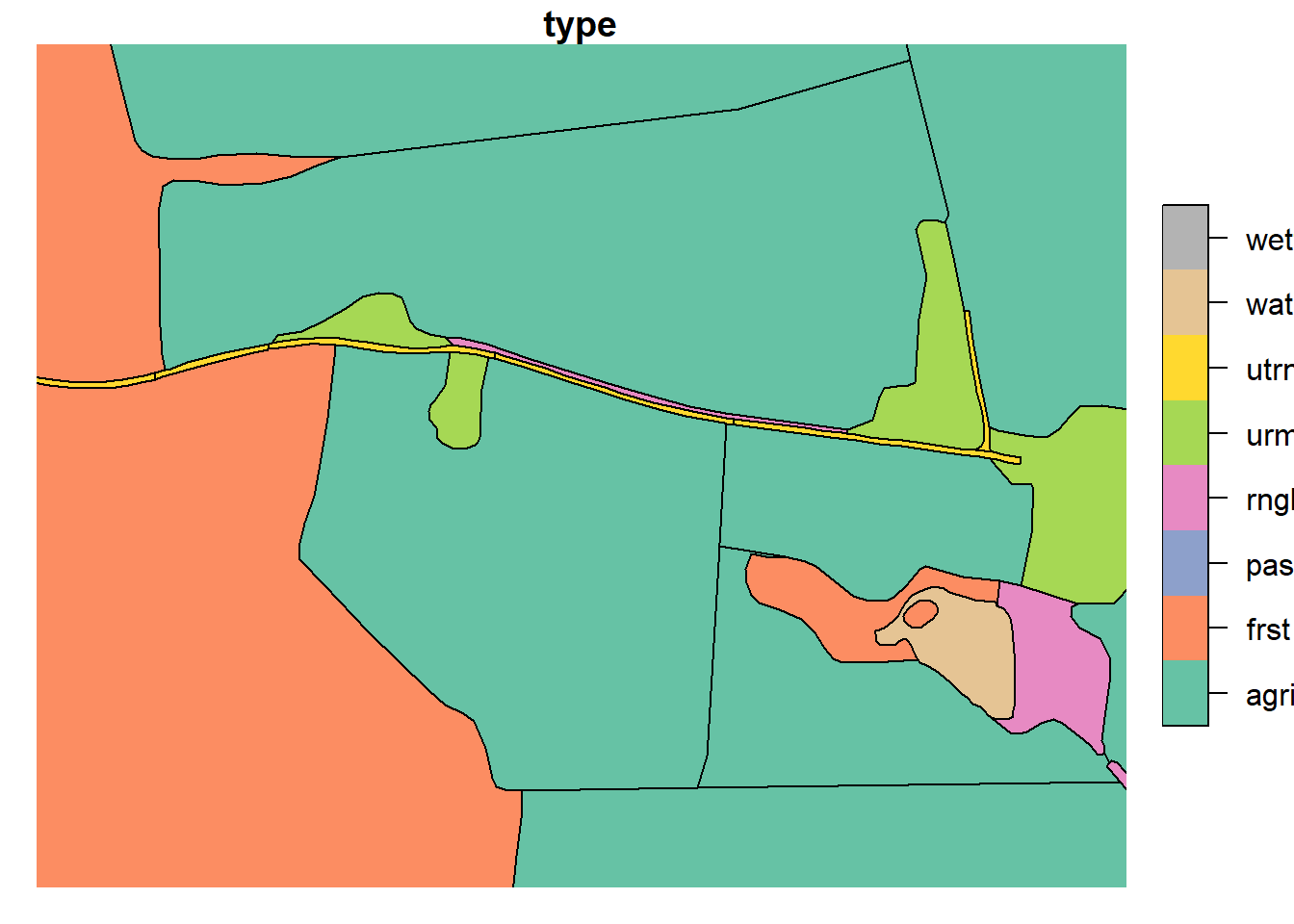
plot(lu_simple['type'], xlim = c(601388.5,602807.8), ylim = c(6616711.7, 6615482.1))
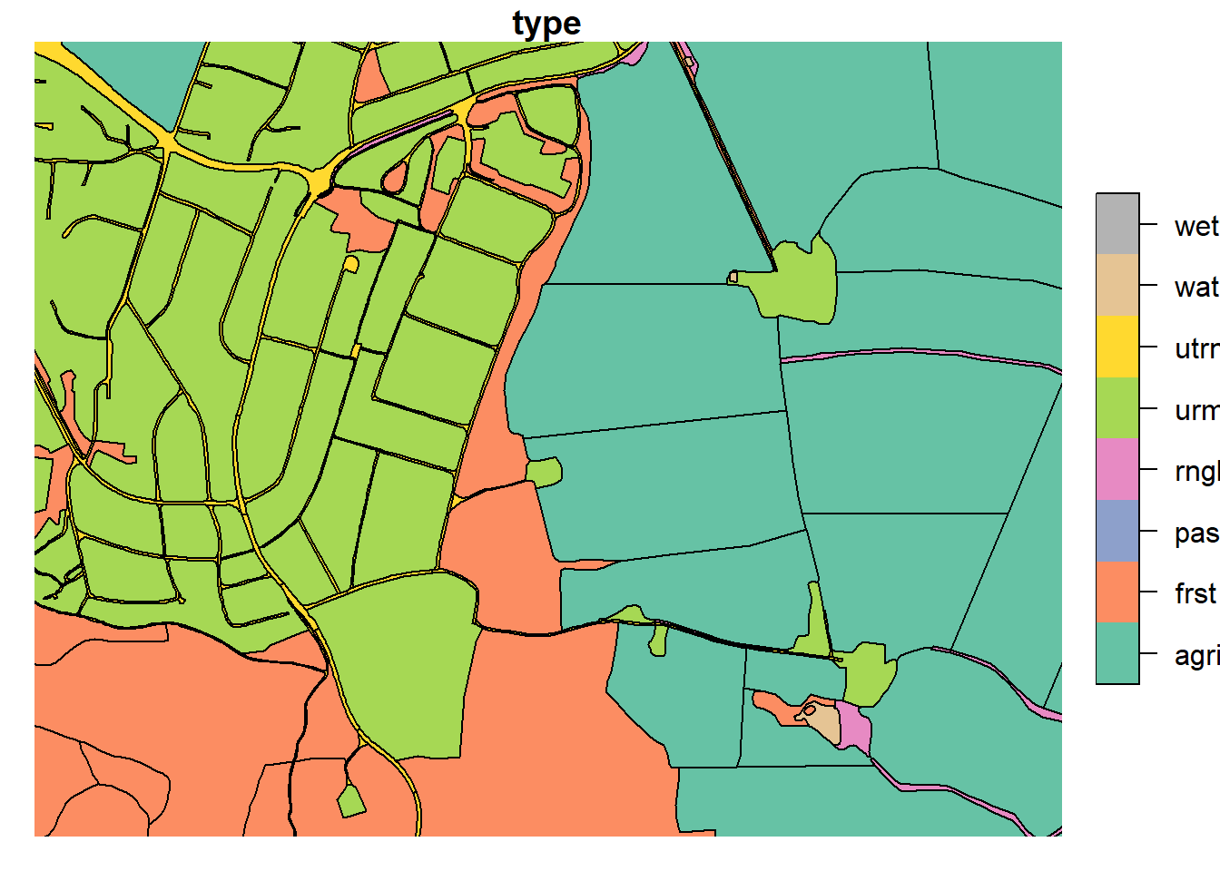
Additionally, all polygons with a perimeter less than <50m (excluding water) or area less than 50m2 were dissolved into their neighboring polygons. Mostly, these were artifacts of infinitely small shapes.
3.4 Splitting Large Polygons
We need to split large polygons into smaller ones, akin to the size of our fields. This is further explained in the OPTAIN modelling protocol, and can be seen in figure 2.6 (Schürz et al. 2022)
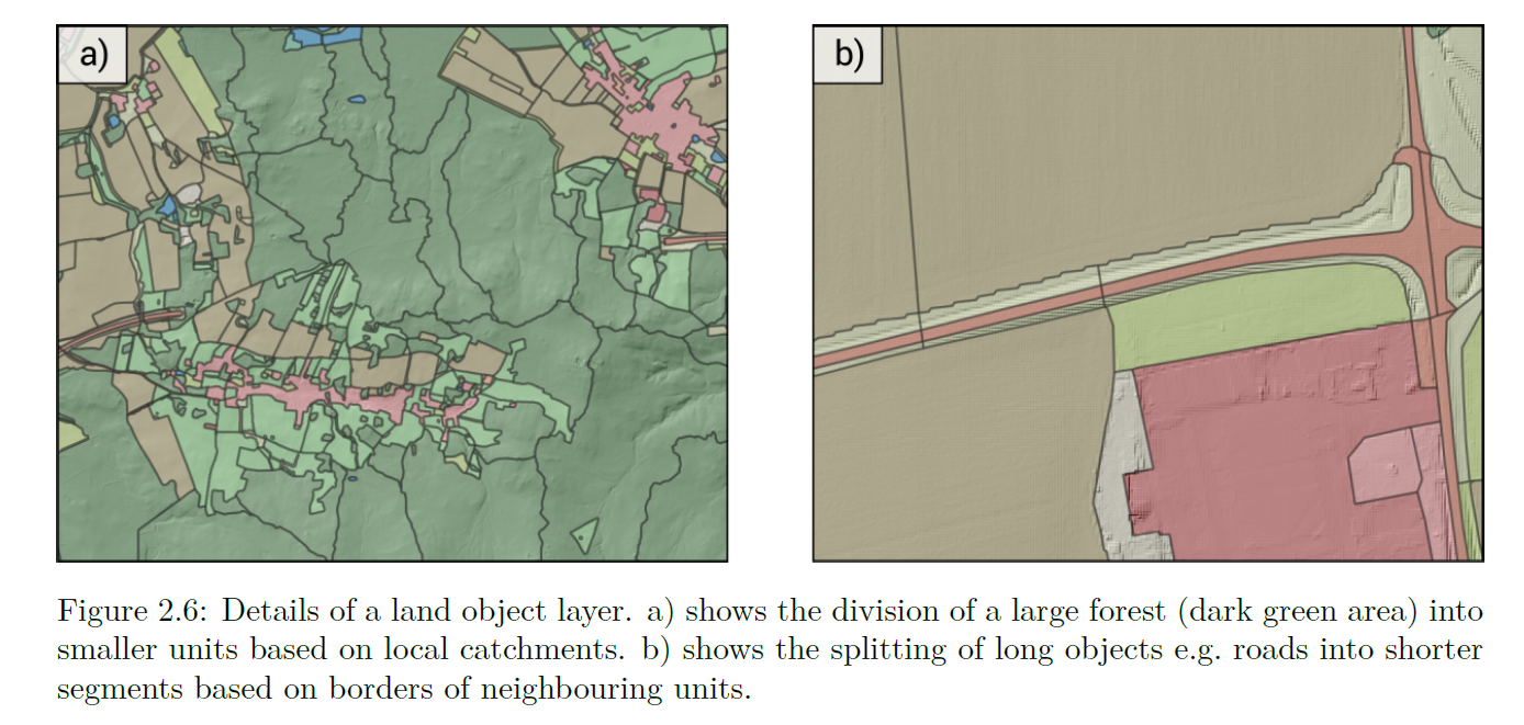
3.4.1 Splitting forests
Forests sometimes can represent huge parts of the landscape, allowing them to rout water between polygons that are spatially very far apart. To prevent this effect, we need to split up our large forests. This was done by intersecting the large forests with the “Løsmasser” map from kart8 (add ref!). This map will later be used to create the soil map. This allows the splits of the forests to match the expected hydrological response. These intersections were subsequently manually adjusted such that any polygons which were too small were re-merged with neighboring.
Any polygons that were large, yet not intersected by “Loesmasser” were manually cut in line with topologically relevant landscape changes. Any polygons “too big” even after intersection were also split. The reference point for “too big” was the average agricultural field size.
par(mar = c(4, 4, .1, .1))
plot(lu_simple['type'], xlim = c(602845.1,604437.2), ylim = c(6616034.3, 6615302.6))
forest_simple <- read_sf("project_data/input/LU/forest/forest_final.shp")
plot(forest_simple['type'], xlim = c(602845.1,604437.2), ylim = c(6616034.3, 6615302.6))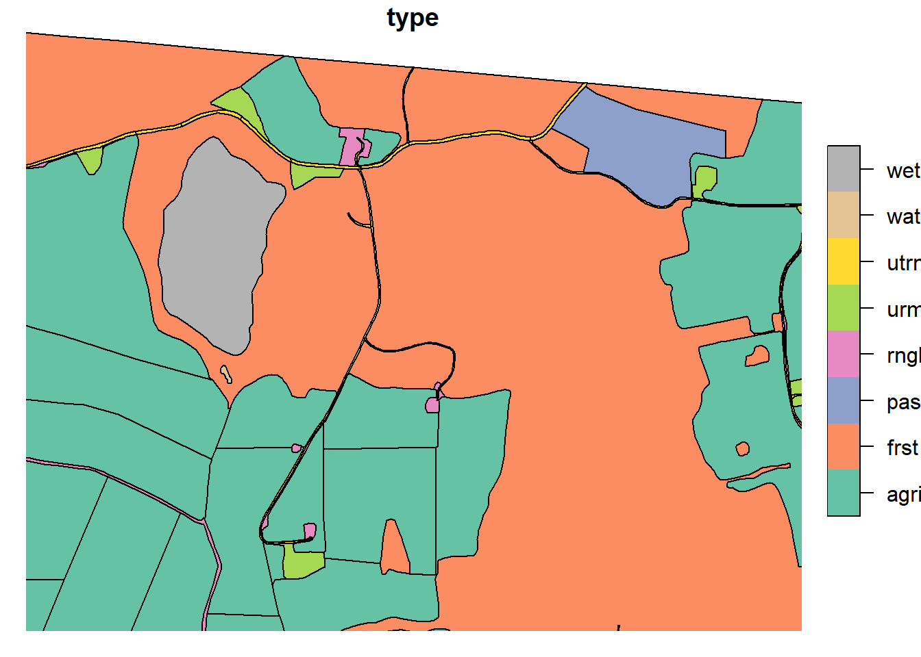
3.4.2 Splitting Roads
Roads were split such that their perimeter did not exceed 400m. Cuts were made in locations topologically relevant to other landscape elements (i.e. at locations where the landscape changes beside the road).
par(mar = c(4, 4, .1, .1))
plot(lu_v2['type'], xlim = c(602074.06,602625.35), ylim = c(6616575.39, 6616364.10))
plot(lu_simple['type'], xlim = c(602074.06,602625.35), ylim = c(6616575.39, 6616364.10))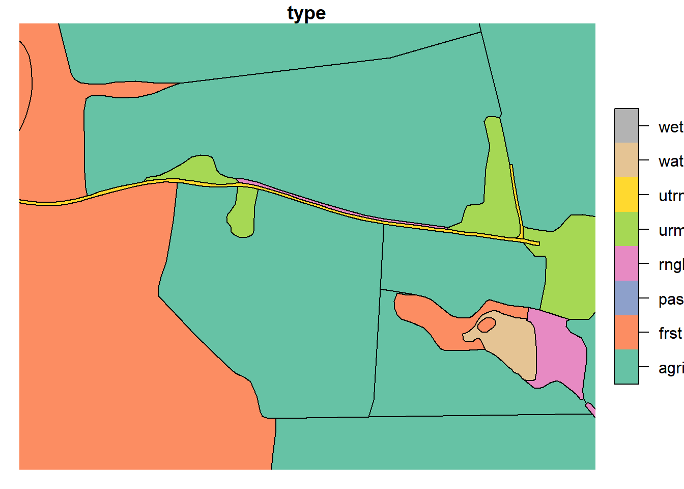
The current geometry of our land use map is now finished. some work needs to be done on the attributes and channels. For now we can save our land use map for further work on the attributes in R. Many small polygons were created in the processing, these were merged with their neighboring polygons using “Eliminate selected polygons” in QGIS.
3.5 Channel network
The channel network must be a GIS line vector layer. it needs fields “id” and “type” where type defines whether it is a surface (cha) or subsurface (sub) channel. Subsurface channels do not receive water from neighboring polygons. In our setup there will be predominantly used for tile drain inlets.
The channel network connects to polygons of type watr. The direction
of the vectors cannot be ignored, it defines the flow of the water.
Splitting a channel (distinct feature with differing ID) is only
necessary at confluence points or at points where measured timeseries
are available. Cross pond splitting is not needed.
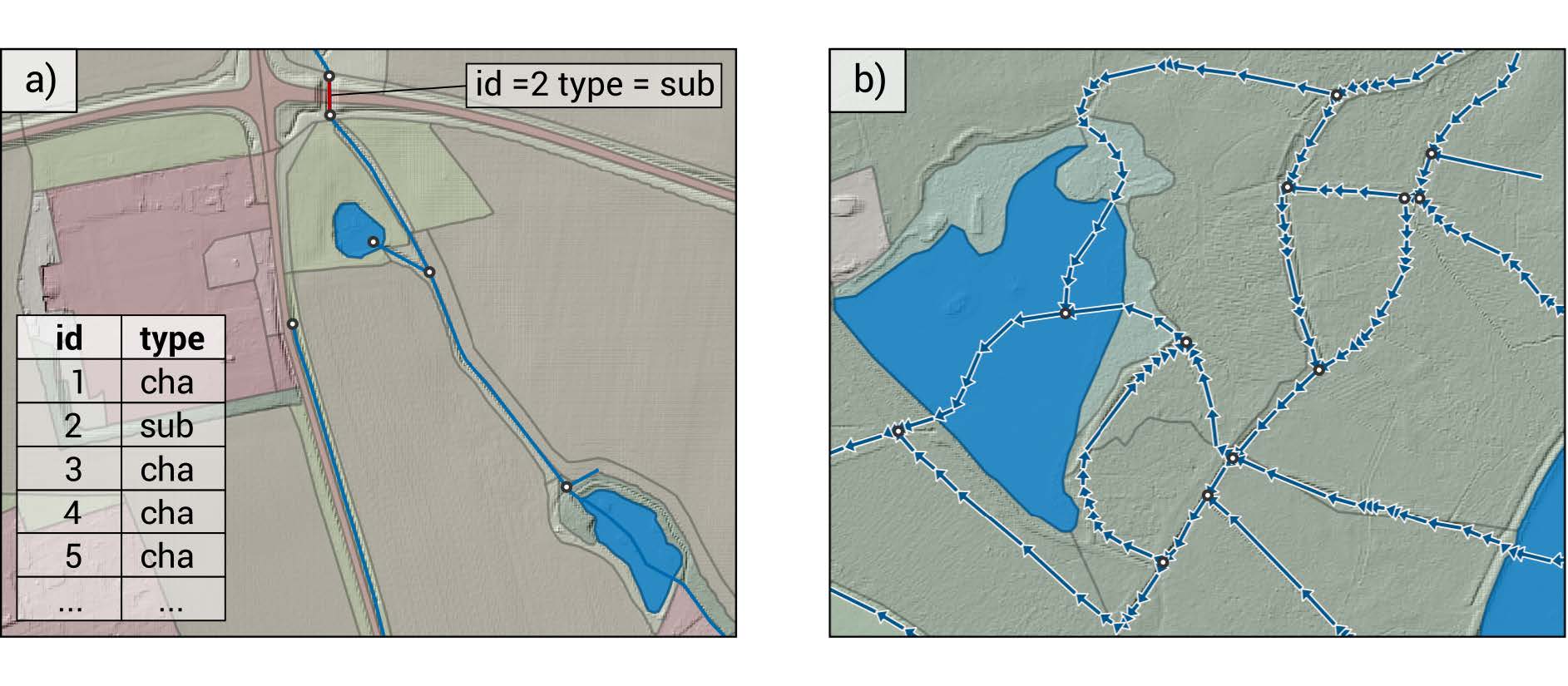
The channel network was created manually using various maps for assistance. In addition to the surface channel network, subsurface channels from tile drain inlets have been added. The locations of these were provided by Robert Barneveld. Here is the provisional result:
tiledrain_inlets <- read_sf("project_data/input/LU/tiledrains/inlets.shp")
channel_network <- read_sf("project_data/input/LU/channels/skuterud_streams.shp")
mapview(channel_network, zcol = "type")+mapview(tiledrain_inlets)+WS TODO: check for road dams
TODO: have an expert check it
TODO: decide on forest channels
3.6 Tile drainage
To incorporate tile-drained on a field-scale in our model setup, we need
to provide buildR with an extra column in our land use map:
drainage. This column will contain the ID of the channel to which
the field is tile-drained into.
As no complete records exist as to what field is drained, and where it drains to, we need to use a proxy. This proxy will be the “drainage class” from the NIBIO “jordmonn” map. You can read more about it here. The classes and their interpretation are as follows:
| Drainage Class | Meaning | Interpretation |
|---|---|---|
| 1 | Self-drained | No tile drainage |
| 2 | Self-draining with wet drafts (?) | No tile drainage |
| 3 | Partially self-drained | Tile drainage |
| 4 | Not self-drained | Tile drainage |
dren_klass <- read_sf("project_data/input/LU/tiledrains/drainage_class_skuterud.shp")
plot(dren_klass['klassenavn'])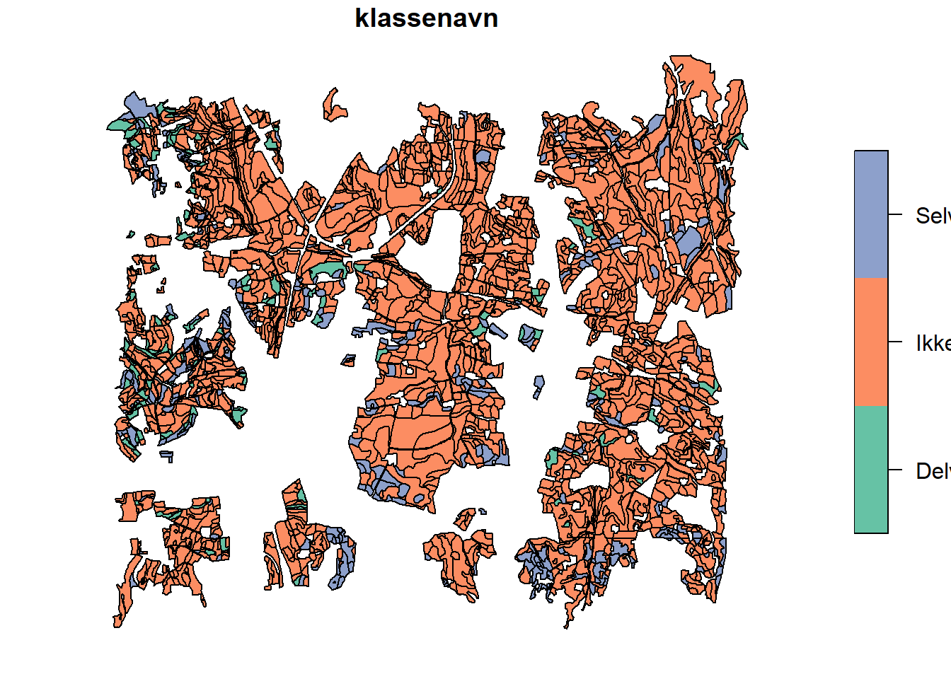
Note, class 2 is not in our catchment area.
To determine which agricultural fields need to be tile drained, we will do a spatial join and add drainage to fields with classes 3 and 4.
lu_skut <- read_sf("project_data/input/LU/lu_skuterud.shp")
dren_klass <- dren_klass %>% st_transform(st_crs(lu_skut))
dren_join <- st_join(lu_skut, dren_klass, largest = TRUE)## Warning: attribute variables are assumed to be spatially constant throughout
## all geometriesdren_join<-dren_join %>% filter(type == "agri")
dren_join$klasse <- dren_join$klasse %>% as.character()
mapview(dren_join, zcol = "klasse")As we can see, all but 6 fields are drained. We will determine which the sub-basins of each defined channel and check which fields fall into that basin. These fields will be assigned to that channel.
channel_network <- read_sf("project_data/input/LU/channels/skuterud_streams.shp")
# don't ask me how or why this works. Point is, it does.
# sample = 0 creates points at the start of each line.
# sample = 1 creates points at the end of each line.
nodes <- st_line_sample(channel_network, sample = 0) %>% st_as_sf()
nodes <- st_transform(nodes, crs(channel_network))
# attaching channel IDs to the points
nodes <- st_join(nodes, channel_network, join = st_touches) %>% st_difference()
nodes <- st_cast(nodes, "POINT")## Warning in st_cast.sf(nodes, "POINT"): repeating attributes for all
## sub-geometries for which they may not be constantdem <- rast("project_data/input/DEM/skuterud_DEM.tif")
nodes <- st_transform(nodes, crs(dem))
write_sf(nodes,"project_data/input/lu/tiledrains/channel_nodes.shp")To figure out which field drains into which, we will create sub-basins for each of these points, and assign the fields to the appropriate sub-basin. First they need to be snapped
require(whitebox)
wbt_jenson_snap_pour_points(
pour_pts = "project_data/input/lu/tiledrains/channel_nodes.shp",
streams = "project_data/input/DEM/wbt_intermediates/raster_streams_drained.tif",
output = "project_data/input/DEM/wbt_intermediates/channel_nodes_snapped.shp",
snap_dist = 30
)then we can create the sub-basins
wbt_watershed(
d8_pntr = "project_data/input/DEM/wbt_intermediates/d8_pointer_drained.tif",
pour_pts = "project_data/input/DEM/wbt_intermediates/channel_nodes_snapped.shp",
output = "project_data/input/DEM/wbt_intermediates/channel_node_subbasin.tif"
)
subbasins <- rast("project_data/input/DEM/wbt_intermediates/channel_node_subbasin.tif")
plot(subbasins)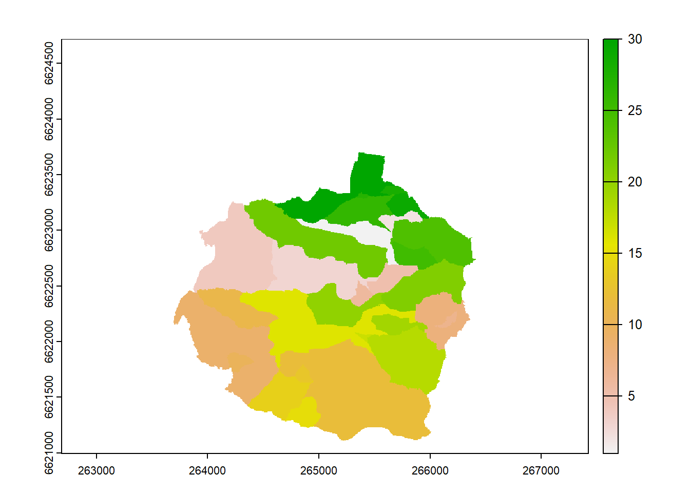
Beautiful. An interactive check:
subbasins_poly <- as.polygons(subbasins) %>% st_as_sf()
# bandaid fix
subbasins_poly$channel_node_subbasin <- subbasins_poly$channel_node_subbasin-1
mapview(subbasins_poly)+mapview(nodes)subbasins_poly <- st_transform(subbasins_poly, crs(lu_skut))
write_sf(subbasins_poly, "project_data/input/LU/tiledrains/channel_subbasins.shp")## Warning in abbreviate_shapefile_names(obj): Field names abbreviated for ESRI
## Shapefile driverNow, we add the ID of the sub-basin to the field that is within it, only if the drainage class is 3 or 4.
lu_skut <- read_sf("project_data/input/LU/lu_skuterud.shp")
join1 <- st_join(lu_skut, subbasins_poly, largest = T)## Warning: attribute variables are assumed to be spatially constant throughout
## all geometries## Warning: attribute variables are assumed to be spatially constant throughout
## all geometrieslu_skut_drain_id <-
join_full %>% mutate(drainage = case_when(
klasse > 2 & type == "agri" & (is.na(SKIFTENR) == FALSE) ~ channel_node_subbasin))
mapview(lu_skut_drain_id, zcol = "drainage")Very nice. Now all we need is to add a unique ID to our polygons for buildR. For agricultural fields this will be the farm+field number, for all others just the type.
3.7 Clipping to Watershed
We only need the polygons within our watershed, so we crop to that. Note: We are using the basin as calculated by BuildR
ws <- read_sf("project_data/skuterud_swat/skuterud/data/vector/basin.shp")
lu_skut_typed<-st_transform(lu_skut_typed, crs(ws))
lu_skut_typed<-st_make_valid(lu_skut_typed)
lu_crop <- st_intersection(lu_skut_typed, ws)## Warning: attribute variables are assumed to be spatially constant throughout
## all geometries## Warning in abbreviate_shapefile_names(obj): Field names abbreviated for ESRI
## Shapefile driverWe now have many tiny polygons at the border which were cut. We can merge them with their largest neighbor. I don’t know how to do this in R yet, so this part will be done manually in QGIS.
# lu_crop2 <- st_cast(lu_crop, "POLYGON")
# lu_crop$AREA <- st_area(lu_crop) %>% as.numeric()
# remove <- lu_crop$AREA < 150
# lu_crop <- vect(lu_crop)
# x <- combineGeoms(lu_crop[!remove,],lu_crop[remove,], boundary = TRUE, dissolve=TRUE)
# mapview(x)
# write_sf(x %>% st_as_sf(), "project_data/input/lu/lu_skuterud_final.shp")Here is the end product:
3.8 Adding unique IDs
We also need a unique numeric id for each polygon:
3.9 BuildR Implementation
# load functions:
fns <- sapply(list.files('project_data/SWATbuildR/functions/', full.names = T), source)
rm(fns)
## Install and load R packages
install_load(crayon_1.5.1, dplyr_1.0.10, forcats_0.5.1, ggplot2_3.3.6,
lubridate_1.8.0, purrr_1.0.0, readr_2.1.2, readxl_1.4.0,
stringr_1.4.0, tibble_3.1.8, tidyr_1.2.0, vroom_1.5.7)
install_load(sf_1.0-8, sfheaders_0.4.0, lwgeom_0.2-8, terra_1.7-3,
whitebox_2.1.5, units_0.8-0)
install_load(DBI_1.1.3, RSQLite_2.2.15)
land_path = "project_data/input/LU/lu_buildRready.shp"
project_path <- 'project_data/skuterud_swat/'
project_name <- 'skuterud'
data_path <- paste(project_path, project_name, 'data', sep = '/')
channel_path <- "project_data/input/lu/channels/skuterud_streams.shp"
project_layer = TRUE## Land layer
land <- read_sf(land_path) %>%
check_layer_attributes(., type_to_lower = FALSE) %>%
check_project_crs(layer = ., data_path = data_path, proj_layer = project_layer,
label = 'land', type = 'vector')
## Check function saves layer into data/vector after all checks were successful
check_polygon_topology(layer = land, data_path = data_path, label = 'land',
area_fct = 0.05, cvrg_frc = 99.9,
checks = c(T,F,T,T,T,T,T,T))## Running topological checks and modifications for the land layer:
##
## Intersection of land layer with basin boundary layer...
## ✔ Intersection completed.
## Analyzing land layer for MULTIPOLYGON features...
## ✔ No MULTIPOLYGON features identified.
## Analyzing land layer for invalid features...
## ✔ No invalid features identified.
## Analyzing land layer for very small feature areas...
## ✔ No small features identified.
## Analyzing land layer for features covered by other features...
## ✔ No covered features identified.
## Analyzing land layer for overlapping features...
## ✔ No overlapping features identified.
## Analyzing land layer coverage with basin boundary...
## ✔ Layer coverage OK.
##
##
## ✔ All checks successful! Saving intersected land layer.## Channel layer
if(!is.null(channel_path)) {
channel <- read_sf(channel_path) %>%
check_layer_attributes(., type_to_lower = TRUE) %>%
check_project_crs(layer = ., data_path = data_path, proj_layer = project_layer,
label = 'channel', type = 'vector')
## Check function saves layer into data/vector after all checks were successful
### altered length fraction to 0...
check_line_topology(layer = channel, data_path = data_path,
label = 'channel', length_fct = 0.00, can_cross = TRUE)
}## Running topological checks and modifications for the channel layer:
##
## Intersection of channel layer with basin boundary layer...
## ✔ Intersection completed.
## Analyzing channel layer for MULTILINE features...
## ✔ No MULTILINE features identified.
## Analyzing channel layer for invalid features...
## ✔ No invalid features identified.
## Analyzing channel layer for very short feature lengths...
## ✔ No small features identified.
##
## ✔ All checks successful! Saving intersected channel layer.### id of the outlet channel
id_cha_out = 27
id_res_out <- NULL
check_cha_res_connectivity(data_path, id_cha_out, id_res_out)## Preparing channel and reservoir features...
## ✔ OK!
## Analyzing connectivity of water object network...
## ✔ No disconnected channels identified.
## ✔ No disconnected reservoirs identified.
##
##
## ✔ Water object connectivity check successful!## Check if any defined channel ids for drainage from land objects do not exist
check_land_drain_ids(data_path)## Load and check DEM raster
dem_path = "project_data/input/DEM/skuterud_DEM.tif"
dem <- rast(dem_path) %>%
check_project_crs(layer = ., data_path = data_path, proj_layer = project_layer,
label = 'dem', type = 'raster')
check_raster_coverage(rst = dem, vct_layer = 'land', data_path = data_path,
label = 'dem', cov_frc = 0.95)
#Save dem layer in data/raster
save_dem_slope_raster(dem, data_path)