Accessing the SeNorge Snow dataset • miljotools

Author: Moritz Shore (moritz.shore@nibio.no)

Date: May, 2026

Introduction

The SeNorge snow dataset is described here:

https://github.com/metno/seNorge_docs/wiki/seNorge_snow

miljotools can access this data using the same functions as for the “SeNorge2018” data.

What follows is a working script on how to access this dataset for a specific shapefile:

Loading Libraries:

require(miljotools)
require(sf)
require(mapview)
require(dplyr)
require(tibble)

Downloading the example catchment:

download.file(url = "https://gitlab.nibio.no/moritzshore/example-files/-/raw/main/MetNoReanalysisV3/cs10_basin.zip", destfile = "cs10_basin.zip")
unzip("cs10_basin.zip")
cs10_basin = "cs10_basin/cs10_basin.shp"
example_polygon_geometry <- read_sf(cs10_basin)
map1 <- mapview(example_polygon_geometry, alpha.regions = .3, legend = F)
map1

Defining coordinate window:

Note, the source is “senorge_snow”!

metnordic_coordwindow(
  area_path = cs10_basin,
  area_buffer = 1000,
  source = "senorge_snow",
  verbose = T,
  interactive = F
) -> cw

## miljo🌿tools > metnordic_coordwindow  >> getting base file from: SeNorge_snow
## miljo🌿tools > metnordic_coordwindow  >> basefile downloaded. 
## miljo🌿tools > metnordic_coordwindow  >> Loading and projecting shapefile... 
## miljo🌿tools > metnordic_coordwindow  >> geometry detected: sfc_POLYGON
## miljo🌿tools > metnordic_coordwindow  >> buffering shapefile:  1000 m
## miljo🌿tools > metnordic_coordwindow  >> calculating coordinate window... 
## miljo🌿tools > metnordic_coordwindow  >> coordinate window is: xmin=341 xmax=350 xmin=163 ymax=179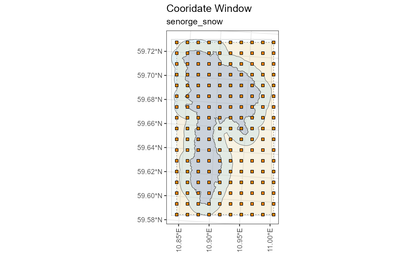

Choosing a variable:

senorge_snow_var = "swe"

SeNorge Snow uses different names for variables depending on whether they are stored in the file name, or within the ncdf4 file itself. This is quite annoying and requires a recoding of the variable name, which can be done using the code below:

senorge_snow_variables <- c("fsw", "lwc", "qsw", "qtt", "sd", "sdfsw", "ski", "swe", "swepr")
senorge_snow_variable_inner <- c("snow_amount","snow_liquid_water_content","snow_melt",
                                   "runoff_amount","snow_depth","snow_depth", 
                                   "snow_condition","snow_water_equivalent",
                                   "snow_water_equivalent_percentage")
snow_recode <- tibble::tibble(outer = senorge_snow_variables, 
                              inner = senorge_snow_variable_inner)


inner_var <- dplyr::recode_values(x = senorge_snow_var,
                                  from = snow_recode$outer,
                                  to = snow_recode$inner)
inner_var

## [1] "snow_water_equivalent"

Building the download queries.

senorge_buildquery(
  bounding_coords = cw,
  variables = senorge_snow_var,
  fromdate = "2016-01-01",
  todate = "2016-12-31",
  grid_resolution = 1,
  verbose = T
) -> myq

## miljo🌿tools > senorge_snow_buildquery  >> You have a grid of: 9 x 16 (144 cells)
## miljo🌿tools > senorge_snow_buildquery  >> generating urls with a grid resolution of: 1 x 1 km
## miljo🌿tools > senorge_buildquery  >> Returning queries.. (1)

Downloading the queries:

Note the use of inner_var in this function!

senorge_download(
  queries = myq,
  directory =  "senorge_snow_download",
  variables = inner_var,
  polygon =  cs10_basin,
  verbose = F
) -> dldir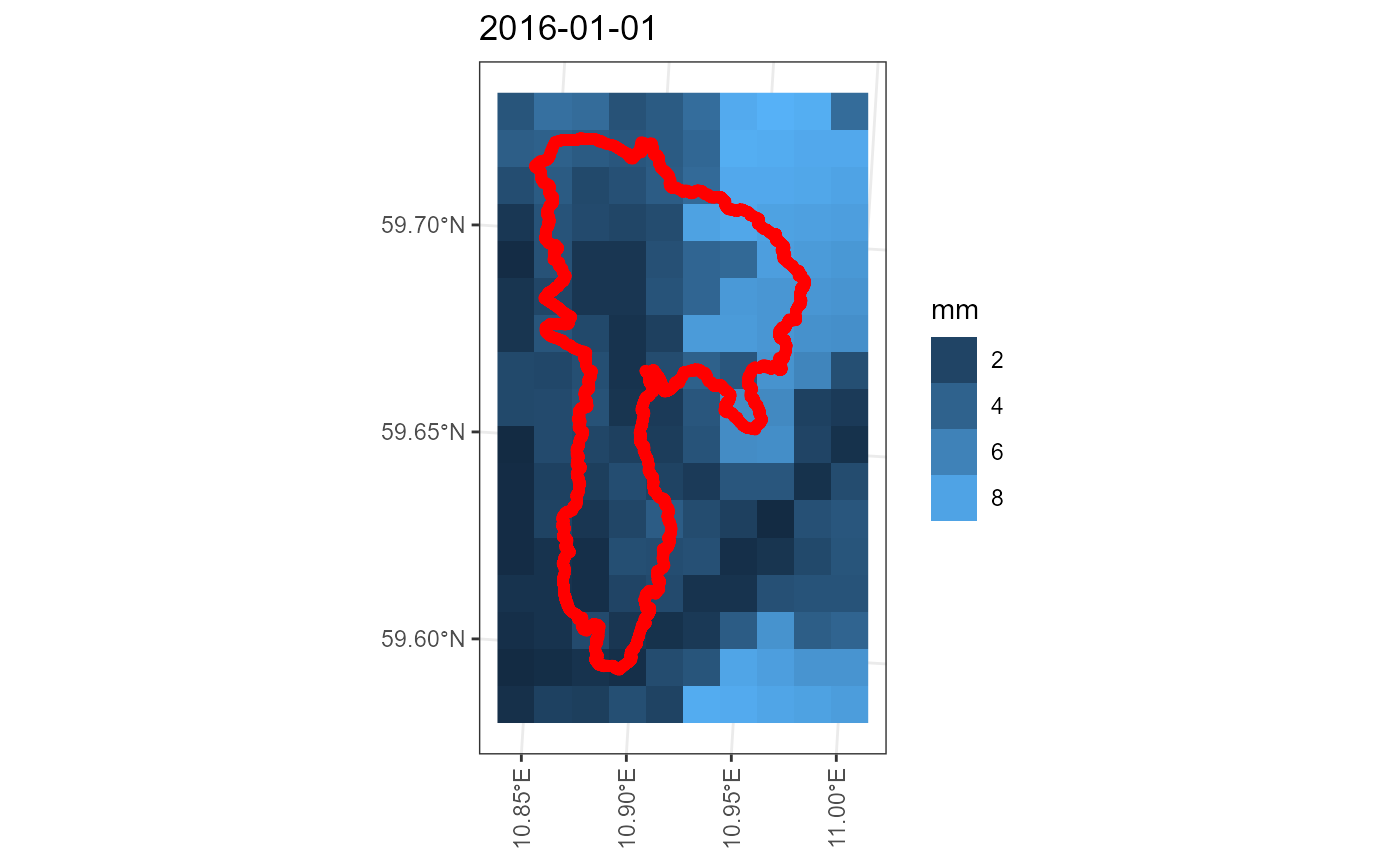

senorge_extract_grid(
  directory = dldir,
  outdir = "senorge_snow_extract",
  area =  cs10_basin,
  variables = inner_var,
  buffer = 250,
  verbose = F,
  map = T
) -> edir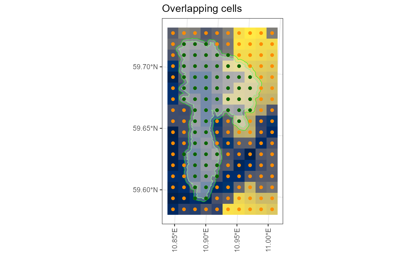

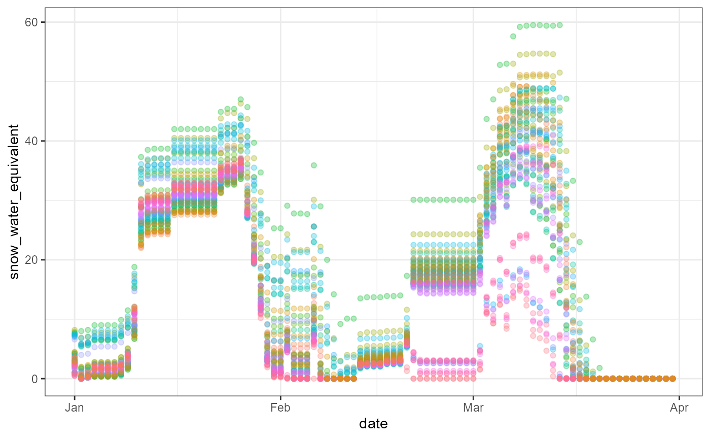
An example analysis using the extracted data:

require(vroom)

## Loading required package: vroom

require(ggplot2)

## Loading required package: ggplot2

list.files(edir, pattern = ".csv", full.names = T) %>% vroom::vroom(show_col_types = F, altrep = FALSE) -> data

data %>% filter(date < "2016-04-01") %>% ggplot() +
  aes(x = date, y = snow_water_equivalent, 
      color = vstation %>% as.factor()) +
  geom_point(alpha = .3) +
  theme_bw() +
  theme(legend.position = "none")