rswap is an R-package designed to help interface and work with SWAP4.2 [1]. It consists of a variety of functions that assist the user in otherwise tedious and repetitive tasks. It is designed to be fully interoperable / backwards compatible with a base SWAP4.2 setup. The scope of the package will hopefully be expanded overtime to include autocalibration / PEST integration, scenario runs, and much more. DISCLAIMER: rswap is very much in development, and therefore not robustly tested, nor extremely stable. use at your own risk, and be critical of the results, for now..
![]()


Table of contents
- Installing rswap
- Running SWAP
- Accessing data
- Visuals
- Model Performance
- Saving model runs
- Comparing model runs
- Modification of Parameters
- Sensitivity Analysis
- SWAPtools Integration
- Miscellaneous functions
- Support and Contributing
- Acknowledgements References
Installing rswap
You can install rswap from GitHub:
# install remotes, if not already present
install.packages("remotes")

remotes::install_github(repo = "moritzshore/rswap", ref = remotes::github_release())

library(rswap)
A useful place to start would be the rswap_init() function. This function creates the “Hupselbrook” example case in the same directory as your swap.exe. It goes on to run the setup, copy in the observed data template file, and plot the results. If this function finished successfully, you know rswap is working properly. Note, rswap only works with SWAP’s latest version: 4.2
project_path <- rswap_init(swap_exe = "C:/path/to/swap.exe")Hint: You can use this
project_pathto run all the following example code on this page!
⚠️IMPORTANT⚠️ Its important to know that rswap never modifies files in your project directory (project_path) unless stated otherwise. Instead all files are copied from project_path to project_path/rswap, modified there, and executed. All results are stored there as well and will be overwritten over time. Remember to save your results if you would like to keep them (save_swap_run(), write_swap_file()), and remember that anything in the project_path/rswap directory is temporary!
Running SWAP
The SWAP model can be run using the run_swap() function. It needs to know where your model setup is located (project_path). The swap.exe must be located in the parent directory of project_path!
run_swap(project_path, autoset_output = TRUE)run_swap() can be further customized with the following parameters:
-
swap_filecan be set to a custom name for your SWAP main file (*.swp) -
autoset_outputcan be enabled (recomended), such that the output of the SWAP model matches your provided observed data -
timeoutsets the max allowed runtime of SWAP -
forceforces a rebuild of the the rswap project from the source files (WIP) -
verbosePrints everything the function does to the console with pretty colors
In parallel?
If you pass more than one project path, these projects will be run in parallel using the run_swap_parallel() function. Using this dedicated function will give you finer control over the parallelized parameters.
Accessing Data
Modelled Data
To read the output of your executed SWAP run, you can use the following command:
modelled_data <- load_swap_output(project_path)load_swap_output() returns two dataframes, daily_output which contains depth wise values of various variables. The other is custom_depth which contains custom variables at custom depths either explicitly altered by the user, or automatically parsed by the autoset_output flag of run_swap(). This dataframe is used widely throughout the package. (more/all results will be added over time)
Observed Data
As rswap heavily revolves around calibration, observed data is of high importance. When running build_rswap_directory() a template observed file will be copied into the project_directory (if not already existing). It is up to the user to fill this file with the appropriate data and column names. Documentation for how to do this is in a companion text file.
To load your observed file, you can use the following command:
observed_data <- load_swap_observed(project_path)Which will return a dataframe of the user-entered observed data
To find out what observed variables you have, as well as their depths, you can use:
get_swap_variables(observed_data)

get_swap_depths(observed_data)
..this can also be filtered by a specific variable by passing variable
Visuals
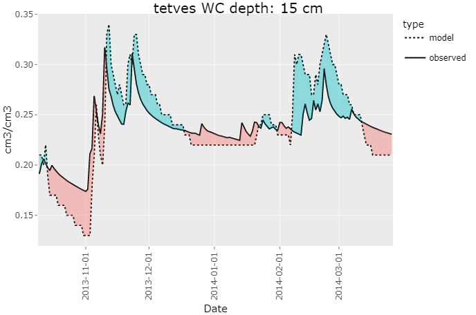
There are a variety of functions used to visualize your SWAP data, such as rswap_plot_variable()
rswap_plot_variable(project_path, variable = "WC", depth = c(15, 40, 70))rswap_plot_variable() can be passed a variable, as well as a vector depth.
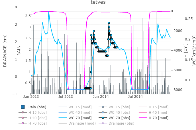
For a more detailed look at multiple variables at once, you can use the rswap_plot_multi()
rswap_plot_multi(project_path, vars = c("H", "WC", "DRAINAGE"))This function can be passed up to 3 variables, and will display them interactively on the same plot. If observed data is available, it will be displayed as well.
Model Performance
A few functions focus on assessing model performance by comparing modelling values to user provided observed values. This functionality is based on the get_swap_performance() function:
get_swap_performance(project_path, stat = "d", variable = "WC", depth = 15)This function is very flexible and can be passed any number of variables, depths, and performance indicators stat (currently supported are select functions from package hydroGOF)
Saving Runs
While calibrating a model it can be useful to keep track of different model runs with different parameterization. rswap aids this process with a variety of functions, such as
save_swap_run(project_path, run_name = "COFRED = 0.35")This function saves your entire model set up in a directory (project_directory/rswap_saved). Once a model run has been saved, it can be compared to other model runs, with the following functions.
Comparing Runs
rswap_plot_compare(project_path, variable = "WC", depth = 15)
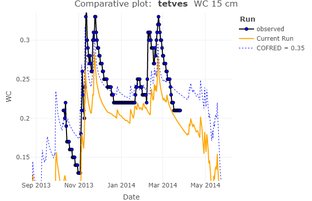
Once again, this function is quite flexible, and can be passed any available variable or depth
You can compare the performance of your various model runs by using the rswap_plot_performance() function.
rswap_plot_performance(project_path, stat = "d", var = "WC", depth = c(15,40,70))
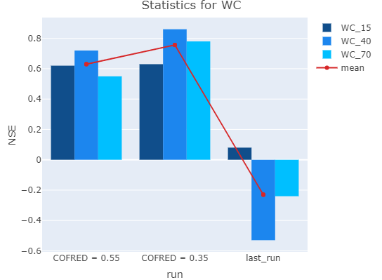
This plot is equally flexible and can be passed any variable and any amount of depths for any supported stat.
Modification of Parameters
Changing of parameters, tables, and vectors of the SWAP main file can be done with rswap. The simple way of doing this is by using the modify_swap_file() function:
modify_swap_file(project_path = project_path,
  input_file = "swap.swp", output_file = "swap_mod.swp",
  variable = "ORES", value = "0.43", row = 2)
This function has many different behaviors depending on which flags are enabled, and which arguments are passed. For more information, check the Details in the help page of the function.
⚠️ If used incorrectly, this function can overwrite your swap file! Check the Details page!
rswap uses a whole set of functions for the reading, altering, and writing of SWAP parameters. While modify_swap_file() covers most use-cases, the underlying functions can be of use as well, for more advanced work flows. You can read more about them in their documentation.
General parameter functions:
# removes any non-essential data from the input file:
clean_swap_file(project_path)
# parses the data to be R-readable:
parse_swap_file(project_path)
# writes the SWAP main file sourced from ".csv" files stored in the rswap directory
write_swap_file(project_path, outfile = "swap_modified.swp")
Parameter specific functions:
param <- load_swap_parameters(project_path)
param <- change_swap_parameter(param, name = "SHAPE", value = "0.75")
write_swap_parameters(project_path, param)
Table specific functions:
tables <- load_swap_tables(project_path)
tables <- change_swap_table(tables, variable = "OSAT", row = 1, value = "0.34")
write_swap_tables(project_path, tables)
Vector specific functions:
vectors <- load_swap_vectors(project_path)
vectors <- change_swap_vector(vectors, variable = "OUTDAT", index = 1, value = "10-jun-2013")
write_swap_vectors(project_path, vectors)
⚠️ You have the choice of passing the value in character format as shown above, to assure FORTRAN compatible format, or you can use the set_swap_format() function, to convert your value to the FORTRAN compatible format.
To run SWAP with the modifications you’ve made to your parameters, you need to make sure you write_swap_file() before running run_swap() – All changes in /rswap/ are temporary until you write your SWAP file!
This functionality is currently only tested for the SWAP main file. Support for the other SWAP input files is coming soon©
Sensitivity Analysis
You can perform a quick sensitivity analysis using rswap using the function check_swap_sensitivity() for example, like so:
check_swap_sensitivity(project_path = "C:/tetves", variable = "OSAT",
                       values = seq(0.32, 0.48, by = 0.01), row = 1,
                       statistic = "NSE", obs_variable = "WC", depth = 15,
                       cleanup = TRUE, autoset_output = TRUE, verbose = TRUE)
This “wrapper” function uses the vectorized behavior of modify_swap_file(), run_swap_parallel() and get_swap_performance() to produce the following graph:
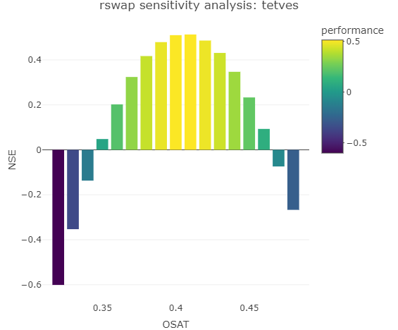
Also returned is a dataframe of the results. This function can be adjusted for any parameter or performance statistic.
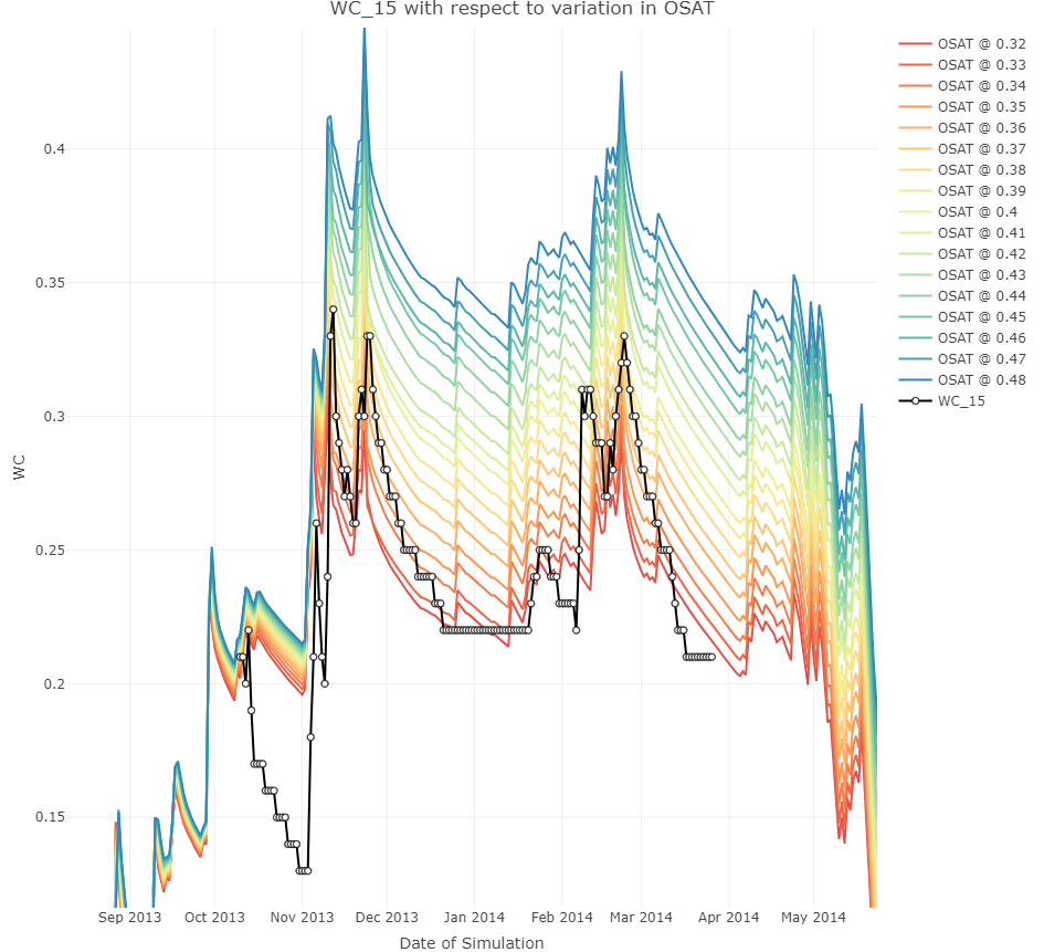
If you would like to see model output response to the varying input, all you need to do is remove the statistic parameter and you will get something like this:
SWAPtools integration
The following features are possible when using rswap with another SWAP-related R-package: SWAPtools
get_swap_format() returns the format of the given parameter, whereas set_swap_format() forces the value of the given parameter into the FORTRAN-required format. These functions rely on data from package SWAPtools. (Over time, change_swap_par() will use these automatically to protect you from incorrect formats)
get_swap_format(parameters = "ALTW")
# [1] "float"

set_swap_format(parameter = "ALTW", value = 5)
# [1] "5.0"
More functionality will be implemented over time.
Miscellaneous functions
The aforementioned functions rely on more basic general functions which, while are designed for internal use, can possibly also be of assistance to the end user. These are listed below.
# Load data
ob_dat <- load_swap_observed(project_path)
mod_dat <- load_swap_output(project_path)

# Filters SWAP data (observed or modelled) by variable and depth
mod_filt <- filter_swap_data(data = mod_dat$custom_depth, var = "WC", depth = 15)
ob_filt <-  filter_swap_data(data = mod_dat$custom_depth, var = "WC", depth = 15)

# Filters and Matches dataframe structure of observed and modelled
data <- match_swap_data(project_path, variable = "WC", depth = 15)

# Melts together all saved runs + current into tidy format
melt_swap_runs(project_path, variable = "WC", depth = 15)
Support and Contributing
If you run into any bugs or problems, please open an issue. The same goes for if you have any suggestions for improvement. If would you like to contribute to the project, let me know! Very open towards collaborative improvement. Fork/Branch off as you please :)
Any OPTAIN case-studies which use rswap are required to bake Moritz Shore a cake using a local recipe from the case-study country.
Acknowledgements
This package was developed for the OPTAIN project and has received funding from the European Union’s Horizon 2020 research and innovation program under grant agreement No. 862756.