Section 8 Field Site Properties

For various use-cases across the modelling project, we will require certain information about the locations of the field sites. This section gathers that information and makes it available to other sections.

run_this_chapter = TRUE

8.1 Determining the HSG group of the logger sites

require(sf)
require(readr)
require(DT)
require(dplyr)
require(mapview)
require(ggplot2)

sf_theme <- theme(axis.text.x=element_blank(), #remove x axis labels
        axis.ticks.x=element_blank(), #remove x axis ticks
        axis.text.y=element_blank(),  #remove y axis labels
        axis.ticks.y=element_blank()  #remove y axis ticks
        )

We load the soil map of the agricultural area.

soil_map <- "model_data/input/soil/soil_map_79.shp"
soil_map_shp <- read_sf(soil_map)

We will crop it by the watershed. Therefore we load the watershed

cs10_basin_path <- "model_data/input/shape/cs10_basin_1m.shp"
cs10_basin <- read_sf(cs10_basin_path)
# reproject
cs10_basin <- st_transform(cs10_basin, st_crs(soil_map_shp))

And crop by by basin. (current not sure of the effect of constant geometry)

st_agr(soil_map_shp) = "constant"
st_agr(cs10_basin) = "constant"
soil_map_shp <- st_intersection(soil_map_shp, cs10_basin)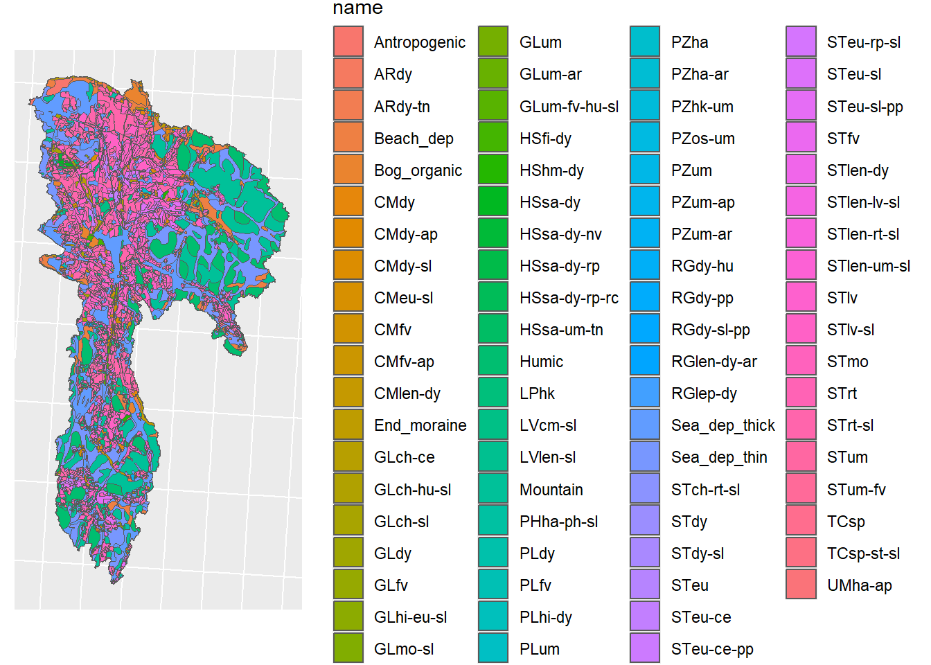

ggplot()+geom_sf(soil_map_shp, mapping = aes(fill = name))+sf_theme

Figure 8.1: Soil map of CS10, in shapefile format

We need information on the soil itself. This is found in our user table. We only need the hydrologic soil group (HSG) HYDGRP, but we will keep the soil depth SOL_ZMX and soil texture TEXTURE just in case

# TODO update this path
usersoil_path <- "model_data/input/soil/usersoil_80.csv"
usersoil <- read_csv(usersoil_path, show_col_types = F)
usersoil <- usersoil %>% dplyr::select(OBJECTID, SNAM, SOL_ZMX, HYDGRP, TEXTURE)

We can combine the two data sets with a left join by soil name

usersoil$name <- usersoil$SNAM


soil_propery_map <- dplyr::left_join(soil_map_shp, usersoil, by = "name")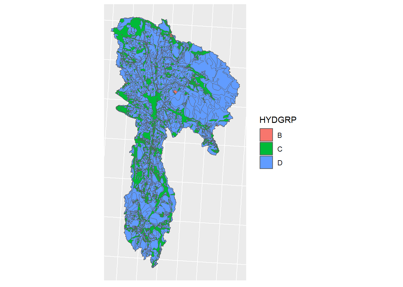

ggplot()+geom_sf(soil_propery_map, mapping = aes(fill = HYDGRP))+sf_theme

Figure 8.2: HSG of CS10

Now we need the locations of the field sites. These are stored as points in the following file:

cs10_field_sites_path <- "model_data/field_sites/geospatial/cs10_field_sites.shp"
cs10_field_sites <- read_sf(cs10_field_sites_path)

We are going to join the attributes using a spatial join

cs10_field_sites <- st_transform(cs10_field_sites, crs = st_crs(soil_propery_map))

field_sites_attr <- st_join(cs10_field_sites, soil_propery_map)

Here is the result:

We have two sites covering C and D, and one site covering B. This covers all existing HSGs in the catchment, which is good. We can save this information in a dataframe.

(UPDATE: with new soil data this is no longer the case)

field_site_attr_df <- st_drop_geometry(field_sites_attr)

datatable(field_site_attr_df)

We will write this into our output folder

write_csv(x = field_site_attr_df, file = "model_data/field_sites/output/field_site_attr_df.csv")

And save our soil property map, and field site points (with attributes)

# TODO fix the weird ID column mess you made
write_sf(field_sites_attr, "model_data/field_sites/output/field_site_attr_map.shp")
write_sf(soil_propery_map, "model_data/field_sites/output/soil_propery_map.shp")