Section 23 Land Object Input (abandoned)

Note, the following pursuit was abandoned. However it shows some initial steps in preparing the land use map.

rm(list=ls())
require(mapview)
require(sf)
require(dplyr)
RUN_THIS_CHAPTER = FALSE

In the OPTAIN project, the land use layer must fulfill the following requirements:

• 100% coverage of the watershed and define all relevant surfaces (Including existing and potential NSWRMs)

• Shape file format, with an id column, a type column defining the land use, and an optional drainage column defining the ID of the channel receiving tile drained water. (see figure REF)

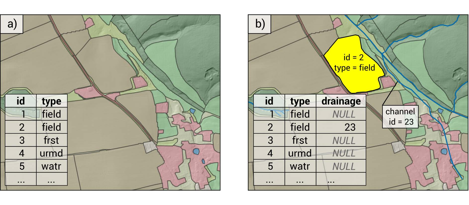
Figure 23.1: Land object polygons with attribute table. a) shows a land layer without tile drainage implemented. b) shows a case where the agricultural field with the land id = 2 has tile drainage activated and drains the tile flow into the channel id = 23 (From REF)

23.0.1 Data sources

23.0.2 Delineation of land objects

Our land use map will remain static, bar the crop rotation we define.

As land use change is not the major focus in OPTAIN, the land unit boundaries for other land uses such as urban areas, open water surfaces, or forest land are static in the land layer.

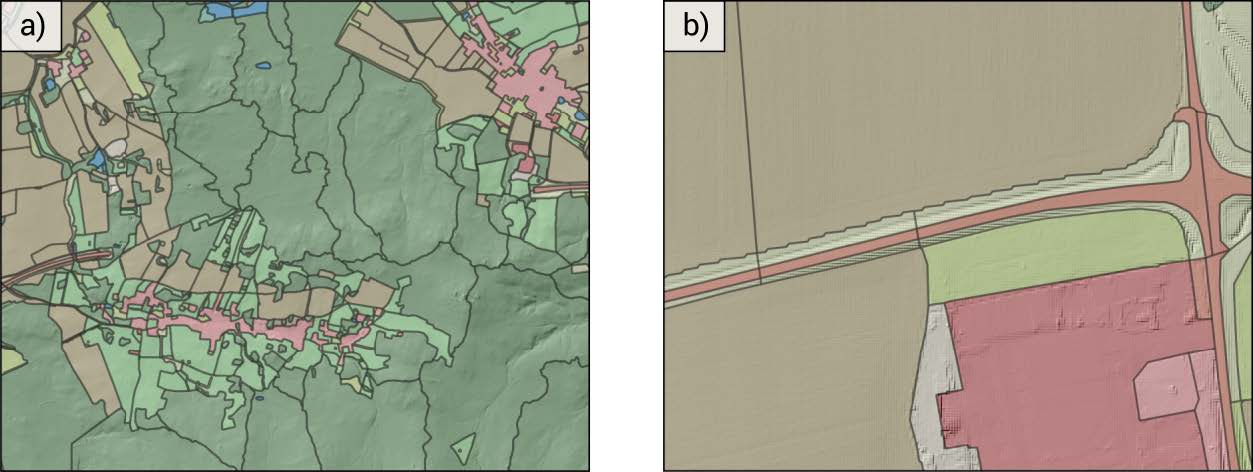
Figure 23.2: Details of a land object layer. a) shows the division of a large forest (dark green area) into smaller units based on local catchments. b) shows the splitting of long objects e.g. roads into shorter segments based on borders of neighbouring units. (From REF)

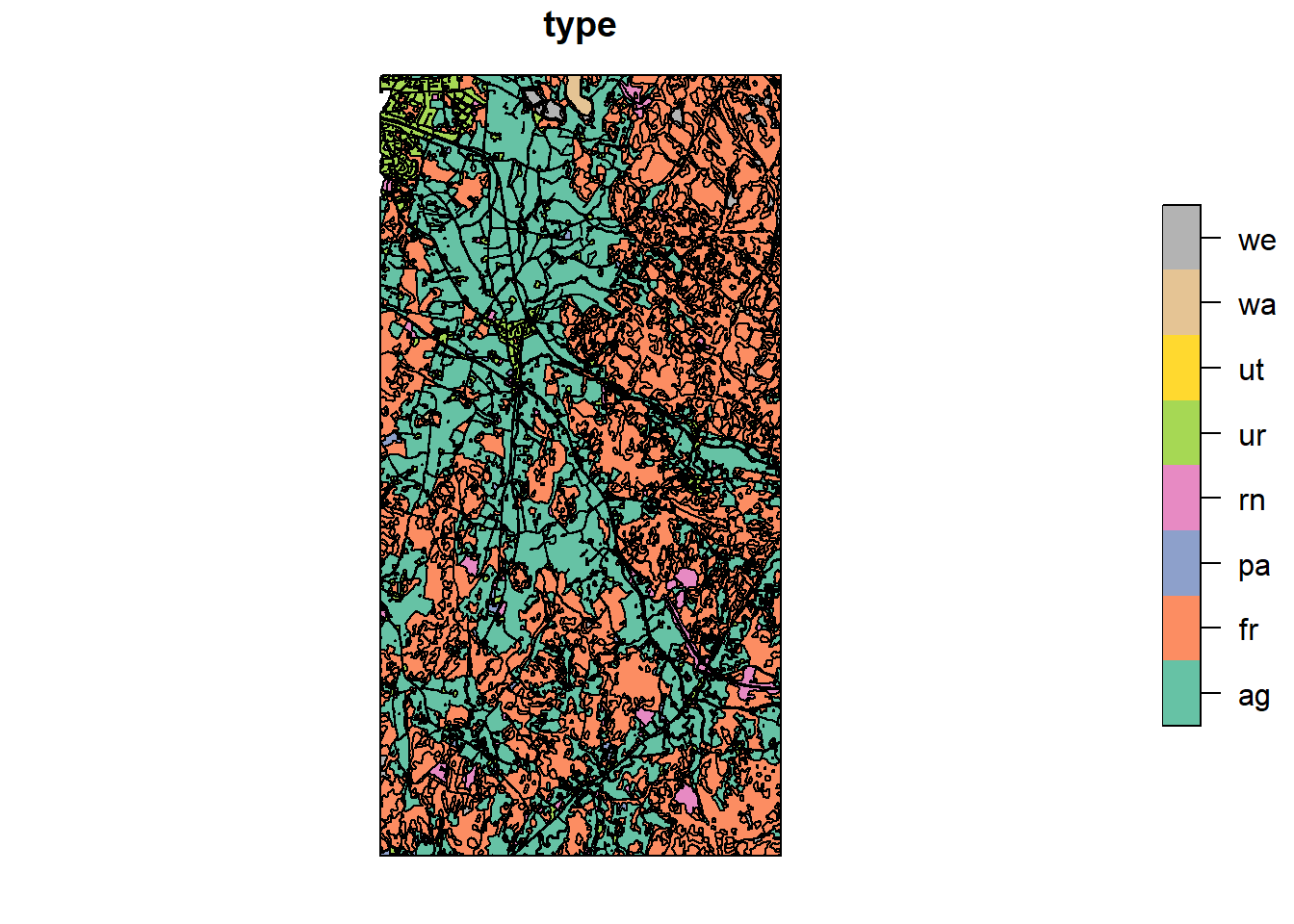
Figure REF shows the level of detail we are aiming for. Notice the agricultural plots are separated, however urban, road networks, and forest land uses are aggregated together, as they are not the focus of OPTAIN.

Each polygon defined here will have negative impact on performance, therefore we need to keep the amount of polygons as low as possible.

“The final land use vector layer should preferably not consist of more than 5,000 - 8,000 polygons”

Also:

“delineated land polygons should not be smaller than two to five times the DEM pixel size.”

Anything smaller can be aggregated.

One important thing to note, is that very large aggregated blocks need to be avoided as well, as they can cause issues with water connectivity (think huge forest polygon with lots of water, strongly connected to just one agricultural field). This is why in figure REF, the large forest and urban blocks are split into smaller parts

Editors note: how does the COCOA connectivity calculation work? Why would a large HRU dump all its water into a single small HRU? doesn’t it / shouldn’t it direct water proportionally to how the actual landscape is?

Here a suggestion from the protocol:

“A practical approach to split large forests into smaller units is to delineate local catchments in a forest and subdivide a forest into its local catchments (see Figure 2.6 a) as an example). Another approach could be to split a forest based on features such as forest roads (similar to the grouping of urban areas) to form blocks of forest land which eventually result in areas comparable to field plots in size.”

Another thing which must be avoided in the land use map are long polygons, as they can cause unrealistic water routing (Think a long road receiving water from 100 HRUs and dumping it all into one HRU at the end of the road).

Editors note: Again, why is this an issue? shouldn’t the COCOA calculation distribute water proportionally?

Suggestion from the protocol (See figure REF for an example)

“To minimize the effect of unrealistic water transfers, splitting such long land objects at edge points of other polygons is considered good practice”

23.0.3 Standing water bodies and the land use type = ‘watr’

Water surfaces require to have the specific label ‘watr’ for their type column.

All water surfaces not connected to the channel network will become reservoirs.

23.0.4 Tile drainage option

Alright enough riff raff lets get started

23.0.5 AR5

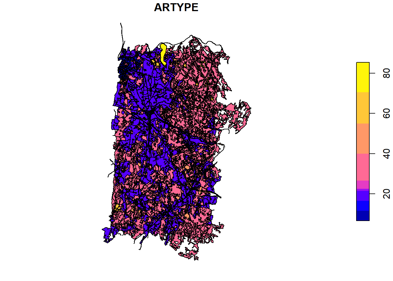
We will use NIBIO’s own AR5 land use map (REF) as a basis for our BuildR ready land use map. You can read more about this map here.

The AR5 shapefile is located here:

ar5 <- "model_data/input/land/ar5_25833.shp"
ar5 <- sf::read_sf(ar5)
plot(ar5)

Lets clean that up a bit, and crop it to our watershed extent

ws <- sf::read_sf("model_data/input/shape/cs10_basin_1m.shp")
ar5 <- sf::st_crop(ar5, ws)

## Warning: attribute variables are assumed to be spatially constant throughout
## all geometries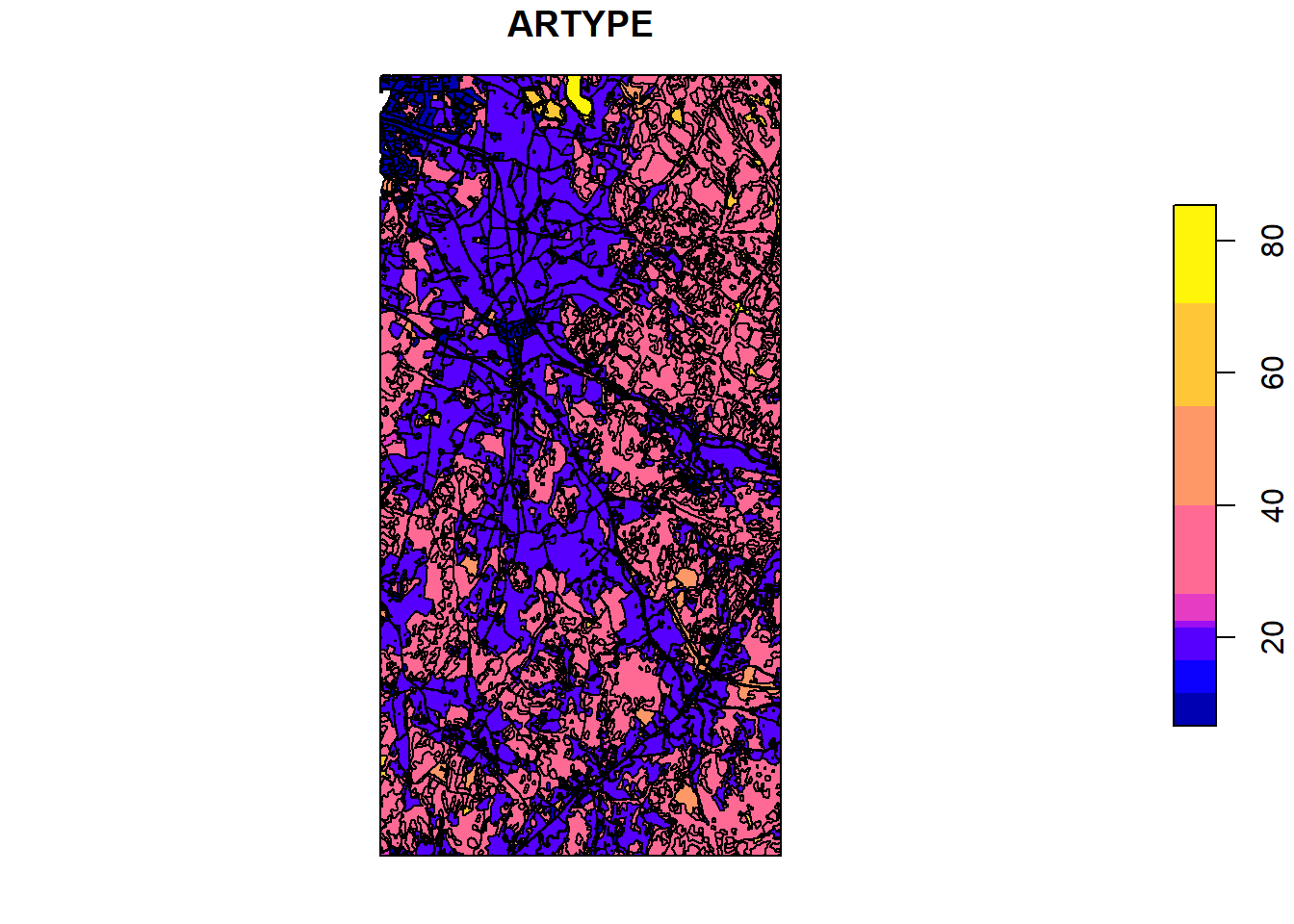

plot(ar5)

Wonderful, now we need to assign the proper land uses to the AR5 codes..

ar5$ARTYPE %>% unique() %>% sort()

## [1] 11 12 21 22 23 30 50 60 81

# TODO figure out the SOMETHINGs

• 11 is is urban which we will define as urml

• 12 is road which we will define as utrn

• 21 is agricultural land, which we will define as agri (note this will have to change later to be field specific)

• 22 is SOMETHING which we will define as past

• 23 is pasture which we will define as past

• 30 is forest, which we will define as frst

• 50 is SOMETHING, which we will define as rngb

• 60 is SOMETHINH which we will define as wetf

• 81 is water which we need to define as watr

ar5$type <- NA

ar5$type[which(ar5$ARTYPE==11)] = "urml"
ar5$type[which(ar5$ARTYPE==12)] = "utrn"
ar5$type[which(ar5$ARTYPE==21)] = "agri"
ar5$type[which(ar5$ARTYPE==22)] = "past"
ar5$type[which(ar5$ARTYPE==23)] = "past"
ar5$type[which(ar5$ARTYPE==30)] = "frst"
ar5$type[which(ar5$ARTYPE==50)] = "rngb"
ar5$type[which(ar5$ARTYPE==60)] = "wetf"
ar5$type[which(ar5$ARTYPE==81)] = "watr"

Now lets have a look at our map again

plot(ar5 %>% dplyr::select(geometry, type))

Very nice, how many polygons do we have right now?

ar5$type %>% length()

## [1] 5887

Wow, that is a lot, since we haven’t even split up our fields yet. Why is it so many? Because currently we have a lot of over complicated geometries:

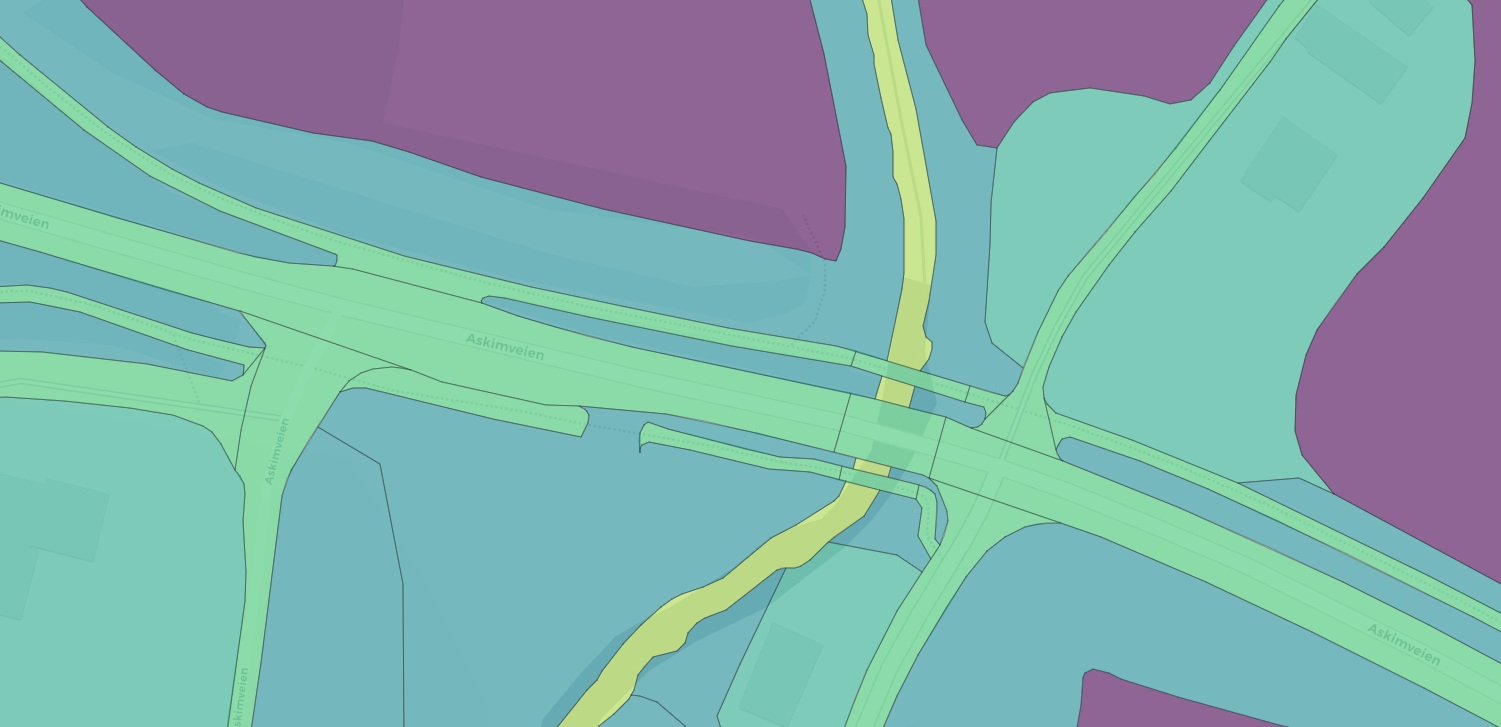
Figure 23.3: Overcomplicated map

We currently don’t need all this extra stuff, so we will merge all polygons of the same type

ar5 <- ar5 %>% group_by(type) %>% summarize()

length(ar5$type)

Just 8, much better. (Don’t worry, we will split these up again when the time comes)

But.. we can do better. This geometry of the urban / road mix is still much too complicated. There is no sense in having the roads within urban areas being separate polygons, therefore we will temporarily merge the two. Later on we will need to manually separate them again, but we would have to do this anyway because we need to manually clip the roads to be shorter, inline with COCOA best practice.

ar5$type[which(ar5$type=="utrn")] = "urml"
ar5 <- ar5 %>% group_by(type) %>% summarize()
length(ar5$type)
plot(ar5)

Figure 23.4: A track and field site with far too many polygons for our model.

Much more simple, however we will need to do some manual pruning. To minimize the manual work, we will now clip this to the basin extent:

ar5 <- st_intersection(ar5, ws) %>% dplyr::select(geometry, type)

## Warning: attribute variables are assumed to be spatially constant throughout
## all geometries

plot(ar5)

And we will split the multi polygons into single polygons to make deleting small polygons easier

ar5 <- st_cast(ar5, "POLYGON")
length(ar5$type)
plot(ar5)

We are already at 1626 polygons, considering we will be burning in field boundaries, splitting roads, urban, and forests, AND burning in all potential measures – this polygon count is going to rise a lot. Therefore we will try to simplify as much as possible in this early stage.

• frst= 375 (probably too few. Need to break up large forest polygons.)

• rngb= 503 (too many, many small shrub polygons)

• urml= 168 (too few, urban areas not split)

• utrn= 0 (too few, roads need to split from urban)

• wetf = 8

• watr = 146 (too many, rivers should not be polygons)

• agri = 392 (too few, need to be broken up into fields)

• past = 34

The manual simplification will be done in QGIS, so lets write out our base map

write_sf(ar5, "model_data/input/land/intermediates/ar5_prep.shp")

We will also use satellite imagery to make expert based decisions on polygon simplification

#rasters <- list.files("model_data/input/satellite/", full.names = T)
#sat_vrt <- terra::vrt(rasters)
#plot(sat_vrt)

23.0.6 Manual Simplification

Simplification work of the base map has been done in QGIS. Something to keep in note for next time: Burn in the potential measures BEFORE you split up large polygons, as the measures will help in splitting things up. And if you do it the other way round, you will end up with many more tiny polygons.

23.0.6.1 Urban Areas

Urban areas were kept rather large, as this study is not focusing on them. The max area was kept at 8 ha.

After simplification, there were 298 urban polygons

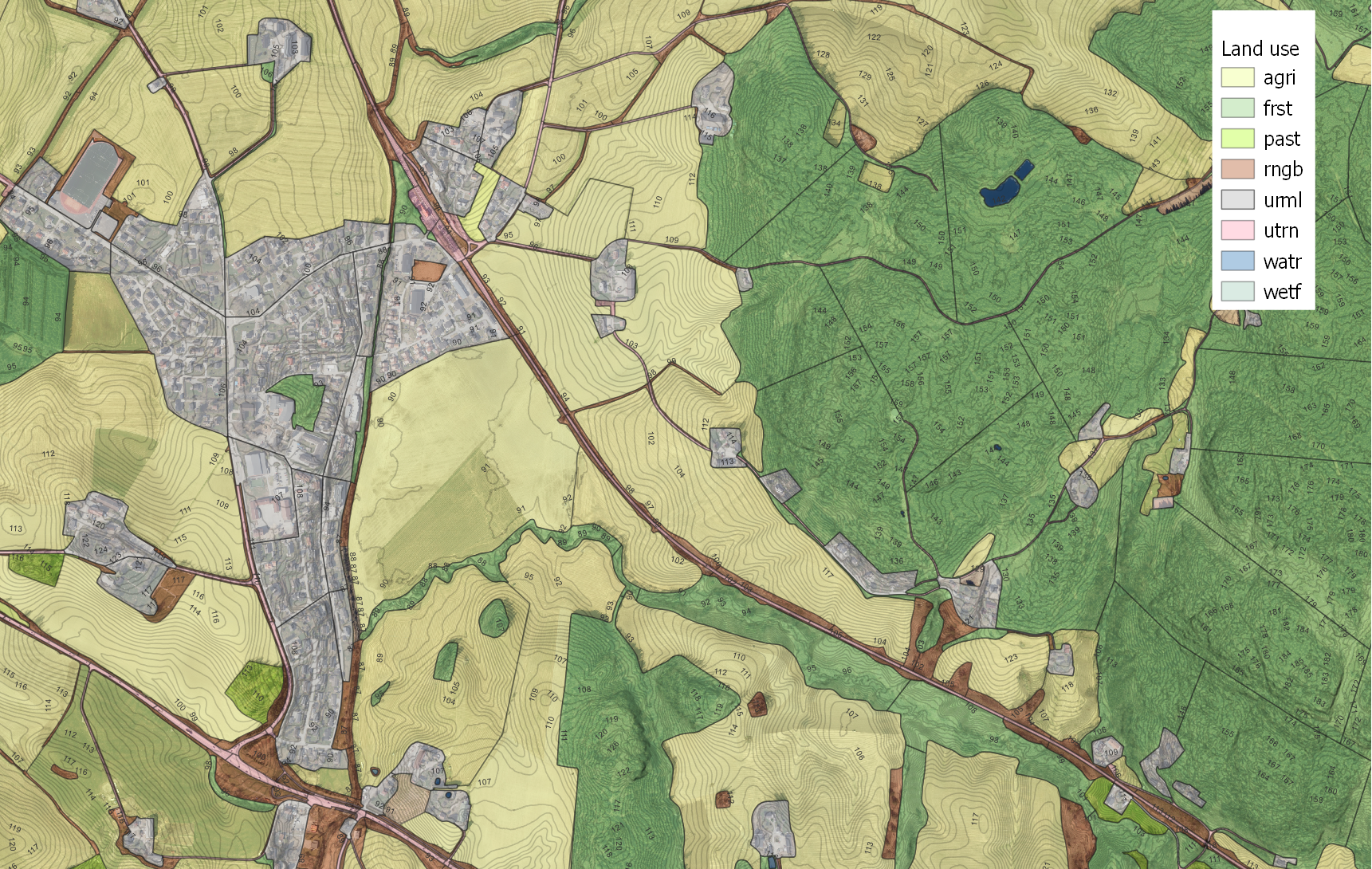
Figure 23.5: The town of Kråstad, urban areas in grey

23.0.6.2 Roads

The road network within urban areas was removed. The remaining road network was split up to maintain a max perimeter of 600m.

After simplification, there were 598 road segments

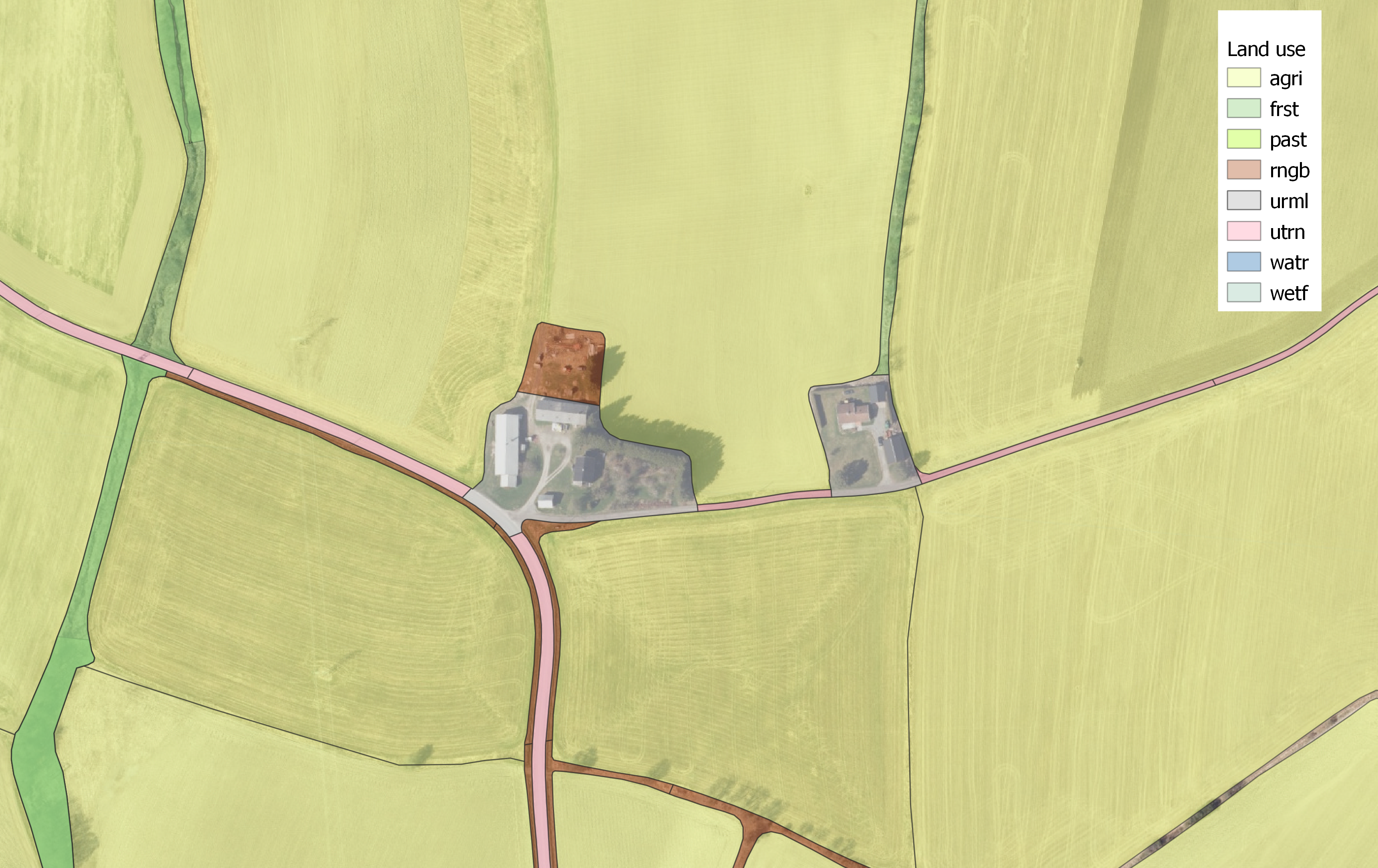
Figure 23.6: Roads (in orange) limited to 600 m perimeter, and removed in urban areas

23.0.6.3 Forests

Forests polygons remained rather large, with area limited to 15 hectares. Odd-shaped polygons were avoided. The DEM was considered while splitting up the large forest polygons, to allow for realistic flow calculations.

After simplifications, 550 forest polygons exist.

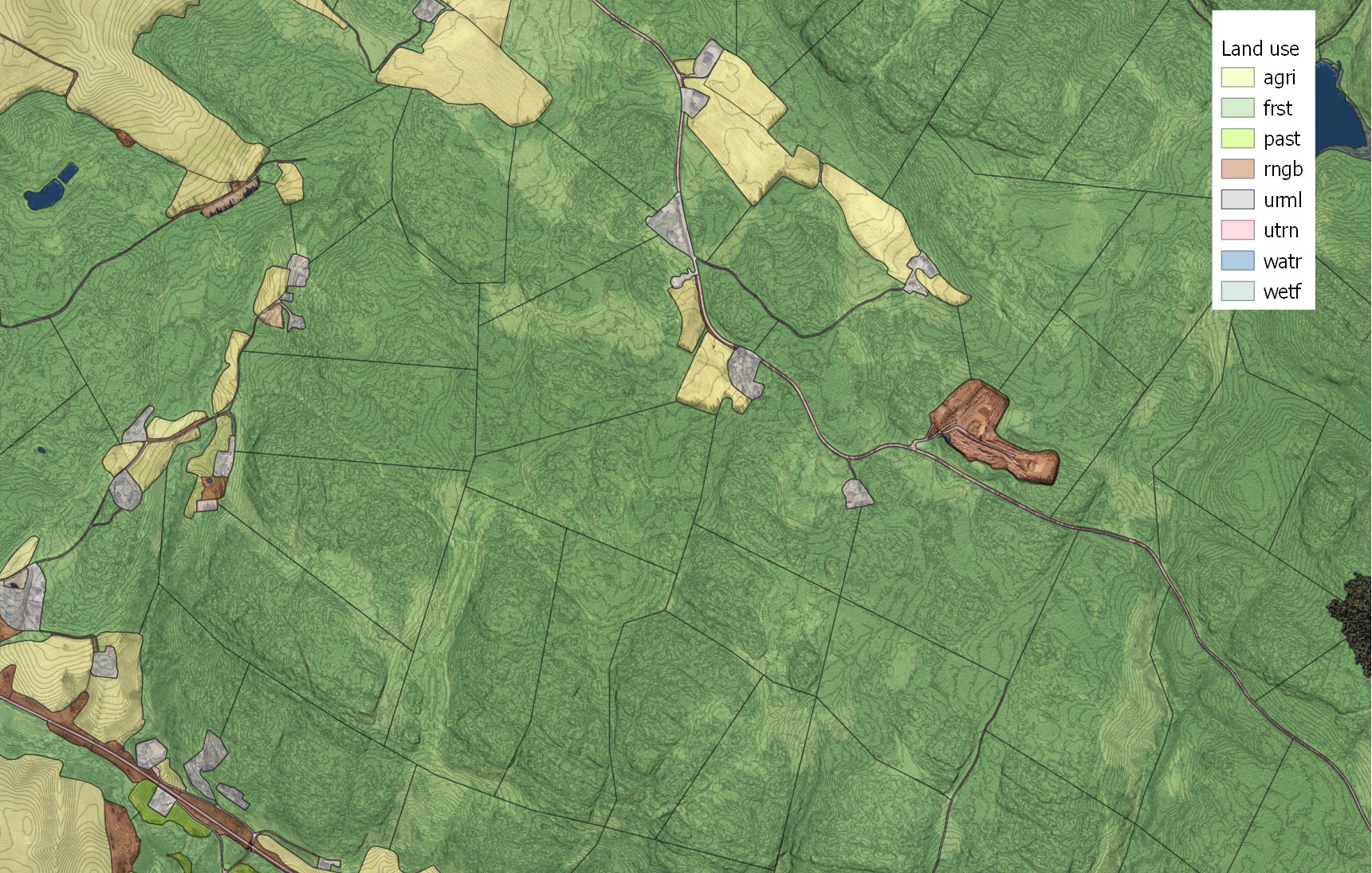
Figure 23.7: Forest polygons, with a DEM hillshade

23.0.6.4 Agricultural Fields

Fields were intersected by the Norwegian real estate register (“matrikkel”). Due to the mismatching of the two data sets (AR5), many tiny polygons were created. These were eliminated. It was attempted to merge fields with less than 3 ha, however some were in reality that small and could not be removed. The smallest field is currently 0.05 ha, however further reductions might be made when all layers are recombined.

After simplification, 468 field polygons exist.

TODO: find source of map

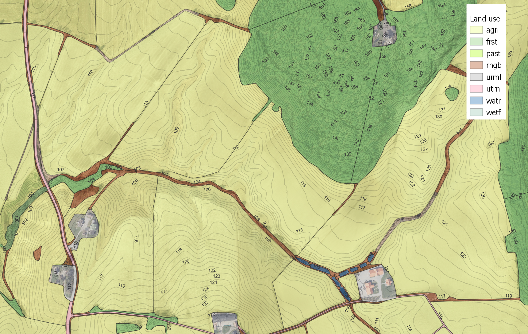
Figure 23.8: Field borders of the agriculutral fields.

23.0.6.5 Shrub land

Shrub lands, as with the road network, were limited to a 600m perimeter. This only applied to long and thin polygons, all others were kept at the approximate size of the agricultural fields.

After simplification and cutting, 864 shrub polygons exist.

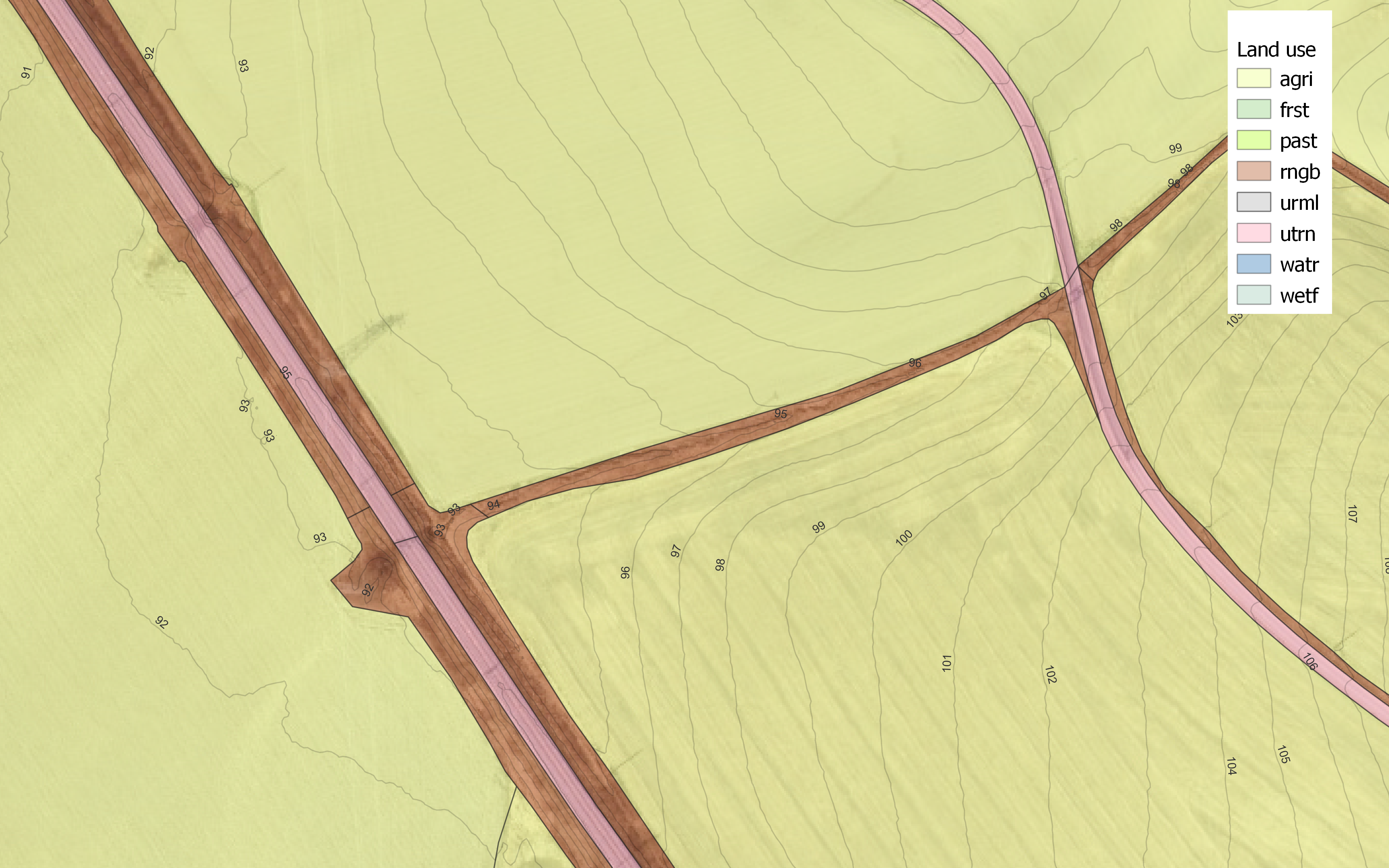
Figure 23.9: Shrubland segmentation

We now total 2901 features. After further simplification we get this down to 2867.

status: 800+ misalignment. need to see how to merge correctly.

NEXT:

• check fields, only keep relevant column

• Prune every small thing you can!!!

• assign drainage

• potential measures

• Prune again!!!

• channels

• Point sources locations?

• Aquifer Objects