Section 3 Weather Input

run_this_chapter = FALSE

3.1 Loading Data

To add weather data to our SWAT project, we will use svatools (Svajunas, Rets, and Strauch 2023)

update 2024: svatools has been migrated to SWATprepR

3.1.1 Required packages

require(euptf2) # devtools::install_github("tkdweber/euptf2") 
require(svatools) # devtools::install_github("biopsichas/svatools")
require(readr)
require(readxl)
require(sf)
require(mapview)
require(ggplot2)
require(tidyr)

3.1.2 Load in the file(s) and load svatools template

First we load in the template and fill it in with our values and rename it to “cs10_weather_data.xlsx”. This is not done within R. No detailed documentation exists on the source of this data (yet).

There has been some discussion in issue #48

#temp_path <- system.file("extdata", "weather_data.xlsx", package = "svatools")
# /// fill out this template and save "cs10_weather_data.xlsx" ///

We are using the following projection for this project:

# TODO update this when the source files are in UTM33N
epgs_code = 25832

Now we can load it in with Svatools.

met_lst <- svatools::load_template(template_path = "model_data/input/met/cs10_weather_data.xlsx", epgs_code)

## [1] "Loading data from template."
## [1] "Reading station ID1 data."
## [1] "Loading of data is finished."

3.1.3 Proof the station

plot_weather(met_lst, "PCP", "year", "sum")

Checking the location of the station:

basin_path <- "model_data/input/shape/cs10_basin.shp"
basin <- st_transform(st_read(basin_path), epgs_code) %>%
  mutate(NAME = "Basin")

## Reading layer `cs10_basin' from data source 
##   `C:\Users\mosh\Documents\GIT\swat-cs10\model_data\input\shape\cs10_basin.shp' 
##   using driver `ESRI Shapefile'
## Simple feature collection with 1 feature and 1 field
## Geometry type: POLYGON
## Dimension:     XY
## Bounding box:  xmin: 603439.4 ymin: 6607792 xmax: 610984.4 ymax: 6622017
## Projected CRS: ETRS89 / UTM zone 32N

stations <- st_transform(met_lst$stations, epgs_code)
mapview(stations) + mapview(basin)

3.2 Weather Generator

We only have one weather station, which means only one weather generator.

wgn <- prepare_wgn(met_lst, 
                   TMP_MAX = met_lst$data$ID1$TMP_MAX, 
                   TMP_MIN = met_lst$data$ID1$TMP_MIN, 
                   PCP = met_lst$data$ID1$PCP, 
                   RELHUM = met_lst$data$ID1$RELHUM, 
                   WNDSPD = met_lst$data$ID1$WNDSPD, 
                   MAXHHR = met_lst$data$ID1$MAXHHR, 
                   SLR = met_lst$data$ID1$SLR)

## [1] "Coordinate system checked and transformed to EPSG:4326."
## [1] "Working on station ID1:WS_AAS"

write.csv(wgn$wgn_st, "model_data/input/met/as_wgn_st.csv", row.names = FALSE, quote = FALSE)

write.csv(wgn$wgn_data, "model_data/input/met/as_wgn_data.csv", row.names = FALSE, quote = FALSE)

3.3 Adding data to SWAT+

This adds the weather generator and weather stations to our SWAT+ project

db_path <- "model_data/cs10_setup/optain-cs10/optain-cs10.sqlite"
add_weather(db_path, met_lst, wgn)

3.4 Atmospheric Deposition

Instructions and documentation can be found here

Getting the data:

basin_path <- "model_data/input/shape/cs10_basin.shp"
df <-
  get_atmo_dep(
    basin_path,
    start_year = 2010,
    end_year = 2020,
    t_ext = "year"
  )

readr::write_csv(df, file = "model_data/input/met/atmodep.csv")

A plot of the results:

df <- readr::read_csv("model_data/input/met/atmodep.csv", show_col_types = F)
ggplot(pivot_longer(df, !DATE, names_to = "par", values_to = "values"), aes(x = DATE, y = values))+ 
  geom_line()+ 
  facet_wrap(~par, scales = "free_y")+ 
  theme_bw()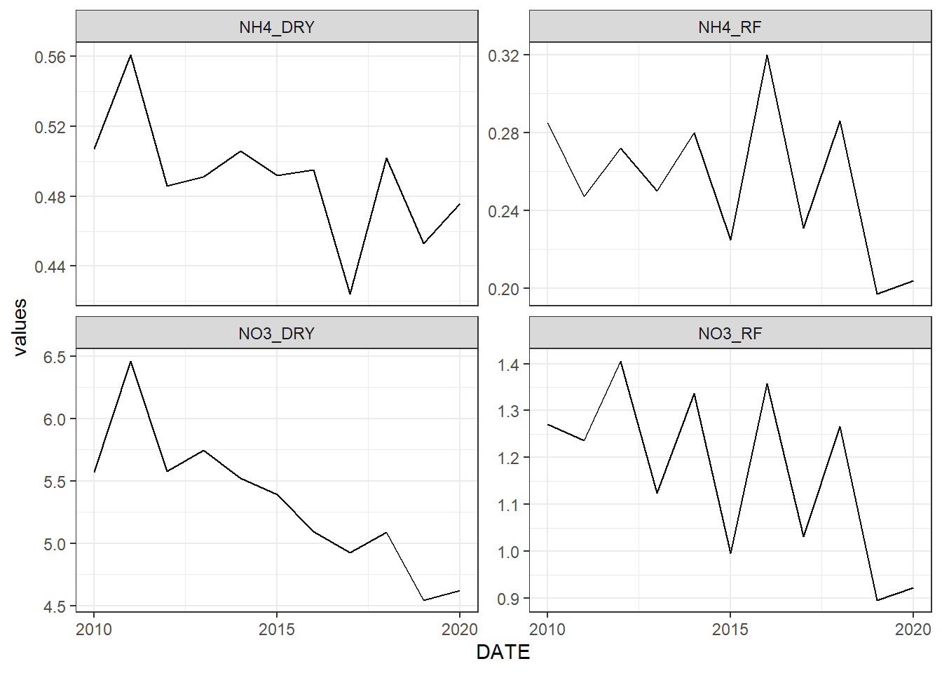

Figure 3.1: Atmospheric Deposition data grabbed by svatools

Adding the data to the SQLITE

db_path <- "model_data/cs10_setup/optain-cs10/optain-cs10.sqlite"
add_atmo_dep(df, db_path)

Big thank you to Svajunas for his svatools package, making our lives much easier!

3.5 Re-analysis Weather

Note: we switched to this dataset in early 2024 as our model performed much better with this dataset. Detailed documentation of this performance increase might someday be added here.

As of March, 2024, our SWAT+ setup uses virtual weather stations derived from a spatially exhaustive dataset of weather data from MetNo’s (met.no) Reanalysis3 project. To do this, our in-house package miljotools was used. You can read more about how this process works, and more about the dataset here

#remotes::install_github(repo = "moritzshore/miljotools", ref = remotes::github_release())
require(miljotools)

## Loading required package: miljotools

The data was sourced and stored in a separate repository:

https://gitlab.nibio.no/moritzshore/metnoreanalysis3-downloads

Therefore the code shown here will only be for documentation purposes and will not actually effect the current project setup.

dir.create("model_data/temp", showWarnings = F)
file.copy(from = list.files("model_data/cs10_setup/swat_input/", full.names = T), to = "model_data/temp", overwrite = T)

##  [1] TRUE TRUE TRUE TRUE TRUE TRUE TRUE TRUE TRUE TRUE TRUE TRUE TRUE TRUE TRUE
## [16] TRUE TRUE TRUE TRUE TRUE TRUE TRUE TRUE TRUE TRUE TRUE TRUE TRUE TRUE TRUE
## [31] TRUE TRUE TRUE TRUE TRUE TRUE TRUE TRUE TRUE TRUE TRUE TRUE TRUE TRUE TRUE
## [46] TRUE TRUE TRUE TRUE TRUE TRUE TRUE TRUE TRUE TRUE TRUE TRUE TRUE TRUE TRUE
## [61] TRUE TRUE TRUE TRUE TRUE TRUE TRUE TRUE TRUE TRUE

The following function gets the (hourly) data. For demonstration purposes, only 3 days worth.

download_folder <- get_metno_reanalysis3(
area = "model_data/input/shape/cs10_basin.shp",
directory = "model_data/temp",
fromdate = "2015-01-01 00:00:00",
todate = "2015-01-03 00:00:00", 
area_buffer = 1500,
preview = T
)

Our SWAT+ setup runs on a daily timestep, so we need daily data:

daily_data_path <-
  reanalysis3_daily(path = download_folder,
                    outpath = "model_data/temp/",
                    precision = 2)

Now with the help of SWATprepR we can add this data to our SWAT+ setup. (excuse the long output)

reanalysis3_swatinput(path = daily_data_path,
                      swat_setup = "model_data/temp/")

These three functions can be consolidated into one workflow with the following function:

swat_weather_input_chain(
  area = "model_data/input/shape/cs10_basin.shp",
  swat_setup = "model_data/temp/",
  directory = "model_data/temp/",
  from = "2013-01-01 00:00:00",
  to = "2022-12-31 00:00:00"
)

Note: as of right now we have unit conversion problems with solar radiation, so we are using our old weather station for SLR.

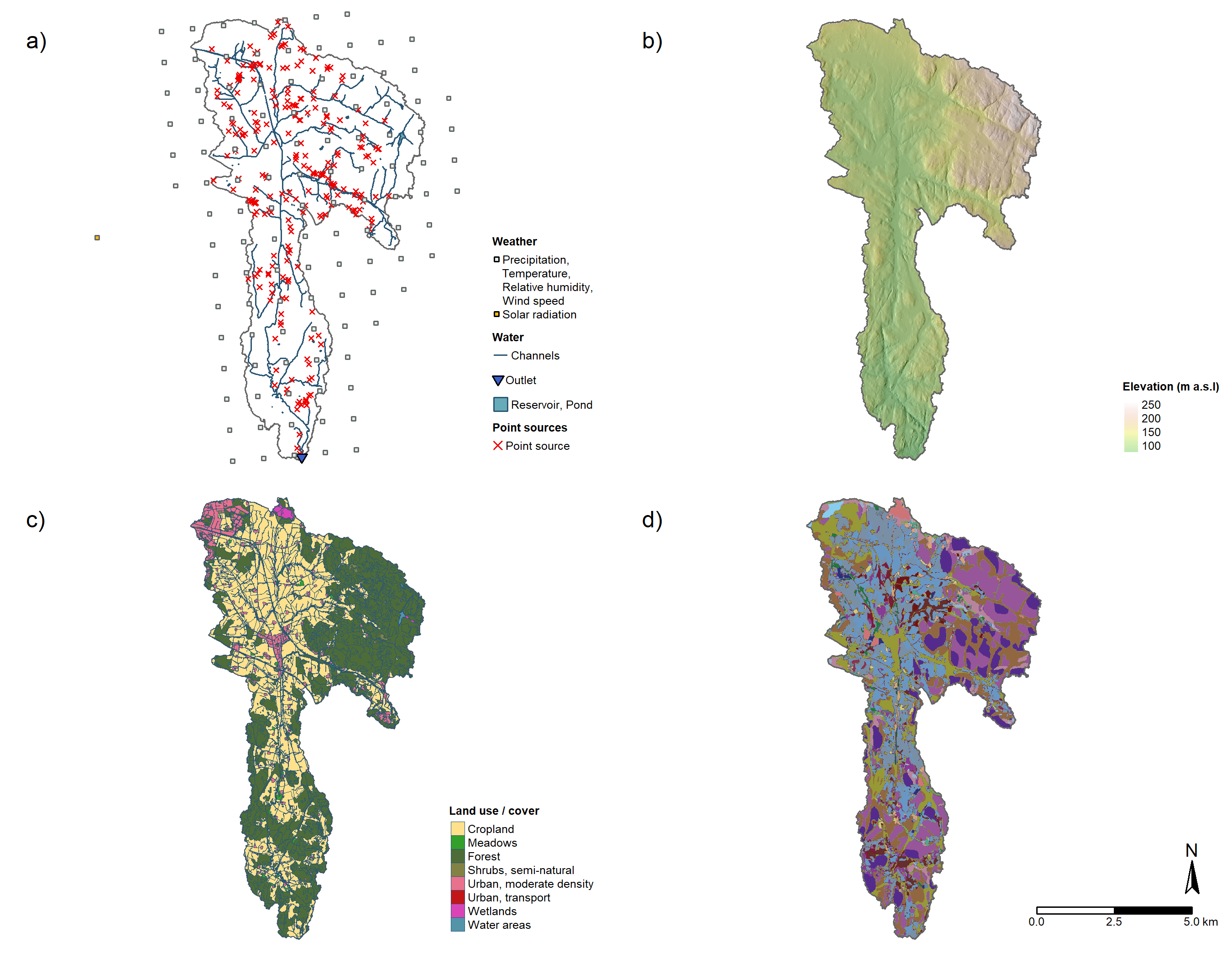
The current state of the weather setup can be seen in panel A :

# clean up our mess 
unlink("model_data/temp/", recursive = T)

References

Svajunas, Ekaterina Rets, and Michael Strauch. 2023. Biopsichas/Svatools: Climate Functions Included. Zenodo. https://doi.org/10.5281/ZENODO.7296033.