Section 1 Input Data Preparation

run_this_chapter = FALSE
run_wbt = FALSE

This Section covers the input data preperation for the SWATbuildR. Some of the documentation of the original creation of the input data has been lost to time.

We will need the following libraries.

# Geospatial:
require(raster)
require(sf)
require(terra)
require(stars)
require(whitebox)

# Plotting
require(gifski)
require(ggplot2)
require(ggrepel)
require(rayshader)
require(mapview)
require(rgl)

# Data manipulation
require(tidyverse)
require(DT)

whitebox::wbt_init(exe_path = "model_data/code/WBT/whitebox_tools.exe")

# Common ggplot theme for simple features
sf_theme <- theme(axis.text.x=element_blank(),
        axis.ticks.x=element_blank(), 
        axis.text.y=element_blank(), 
        axis.ticks.y=element_blank()
        )

For our model setup, we need the following layers, Some of which will be created in this section.

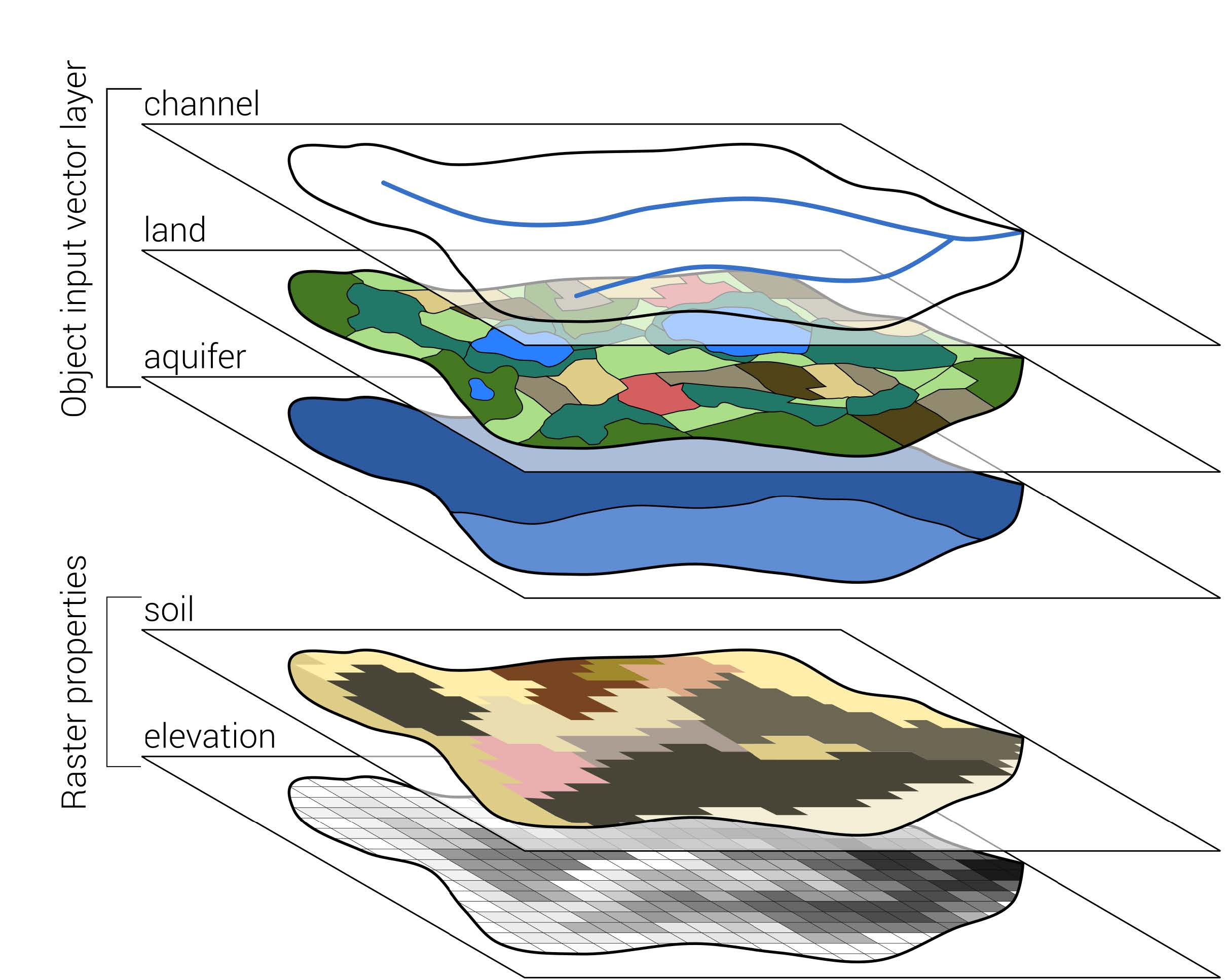
Figure 1.1: Required vector and raster inputs for a SWAT+ model setup with SWATbuildR Schürz et al. (2022)

1.1 Digital Elevation Model

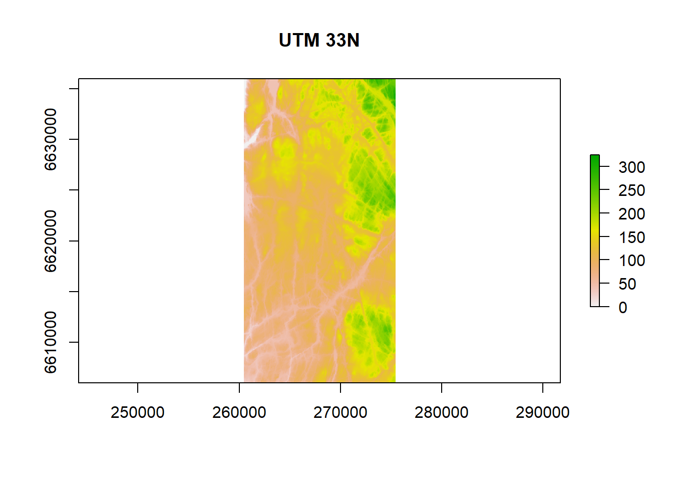
The DEM is sourced from hoydedata.no and has a resolution of 10m. 1m Resolution was available but not used.

dem_path <- "model_data/input/elevation/dtm3_ns_v5.tif"

dem_rast <- raster(dem_path)
plot(dem_rast)

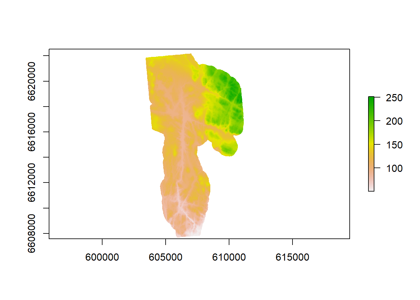
Figure 1.2: CS10 Digital elevation model at 10 meter resolution.

To our knowledge, it has a 10 meter resolution. 1 meter resolution was available but there seems to have been issues with using it. It is definitely preferable to use the 1m DEM as certain important information can be lost with (max allowed resolution) of 10m.

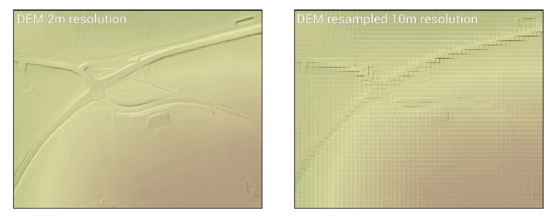
Figure 1.3: An example of a hydrologically effective landscape features being lost due to coarse DEM resolution. From Schürz et al. (2022)

1.1.1 High resolution DEM

From hoydedata.no, the 1M DEM tiles which cover our watershed are

tile_1 <- "model_data/input/elevation/dtm1_33_124_112.tif"
tile_2 <- "model_data/input/elevation/dtm1_33_124_113.tif"

Lets have a look (Don’t mind the low plot resolution, it is to save on computer resources)

tile1_rast <- rast(tile_1)
tile2_rast <- rast(tile_2)

tile1_rasterlayer <- as(tile1_rast, "Raster")
tile2_rasterlayer <- as(tile2_rast, "Raster")

tile1_map <- mapview(tile1_rasterlayer, maxpixels = 1000)
tile2_map <- mapview(tile2_rasterlayer, maxpixels = 1000)

basin_shp <- read_sf("model_data/input/shape/cs10_basin.shp")
basin_map <- mapview(basin_shp)

tile1_map+tile2_map+basin_map

See that line that splits them? We need to combine them and we can do it with a raster mosaic:

rast_collection <- sprc(tile1_rast, tile2_rast)
full_dem <- terra::mosaic(rast_collection)

Lets have a look:

plot(full_dem)

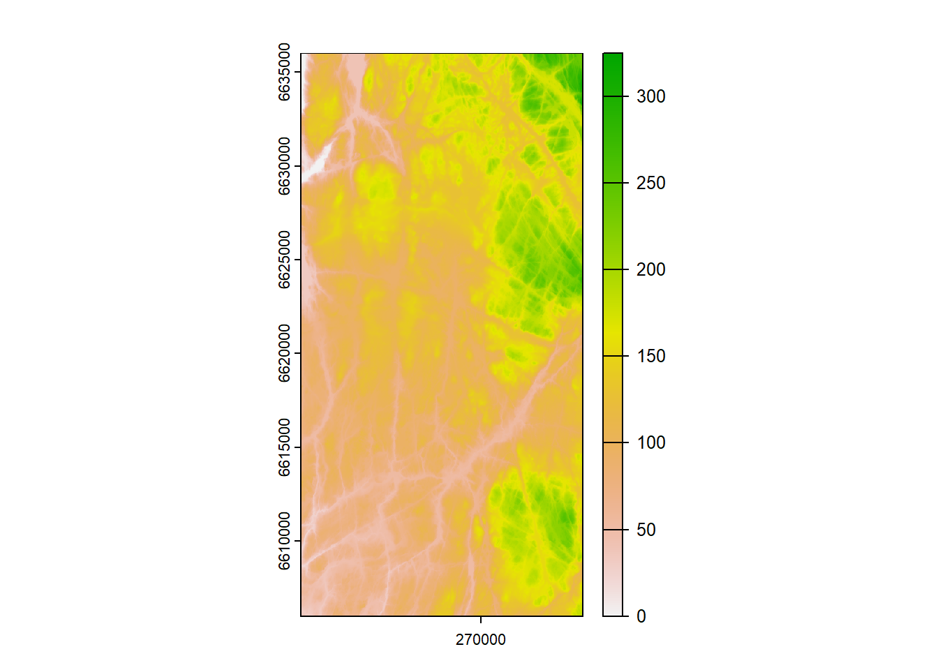
Figure 1.4: One meter digital elevation model for the CS10 area.

How about that basin coverage? (Don’t mind the low resolution, its to save on memory and computation)

dem_layer <- as(full_dem, "Raster")
basin_map+mapview(dem_layer, maxpixels = 1000)

Looks good, lets save it.

writeRaster(full_dem, "model_data/input/elevation/cs10_dem_1m_utm33n.tif",
            overwrite = TRUE)

1.2 Soil Data

For BuildR to generate our soil layer, we need the following:

1. a GeoTiff raster layer that defines the spatial locations of the soil classes (with integer ID values).

 "model_data/input/soil/soil_raster.tif"

2. a lookup table in .csv format, which links the IDs of the soil classes with their names

"model_data/input/soil/soil_lookup_26.csv"

3. a usersoil table in .csv format, which provides physical and chemical parameters of all soil layers for each soil class that is defined in the raster layer and the lookup table. An example soil dataset can be acquired e.g. from the ExampleDatasets folder which comes with an installation of SWAT+.

"model_data/input/soil/usersoil_26_v2.csv"

The documentation for how we created our usersoil is lost to the sands of time, however a OPTAIN-Specific and R-based workflow does exist and can be used. This workflow is based on svatools and is explained here.

Some fragments of our usersoil creation documentation can be found in this file

"model_data/legacy_setup/input_files/soil/UserSoil_Krakstad.xlsx"

1.2.1 High resolution soil maps

A high resolution soil map is required to accurately represent the Hydrologic Response Units (HRUs) used in the OPTAIN project:

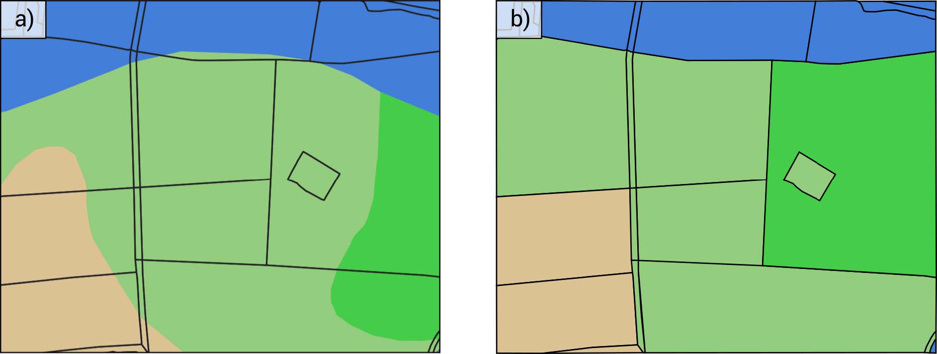
Figure 1.5: Spatially adequate representation of soil heterogeneity on field plot scale. The different colours represent different soil classes. The black border lines represent the boundaries of spatial objects (e.g. agricultural fields). a) the original soil input layer. b) the dominant soil aggregation as performed by SWATbuildR. Schürz et al. (2022)

The use of an extremely detailed soil map is however not recommended:

The use of soil information on a scale which is much more detailed than the scale of the spatial objects in a model setup is however not recommended. It might be difficult to provide parameters to the usersoil table for less common soil types. Moreover, by default SWATbuildR uses the dominant soil class for each spatial object in the model setup process (see Figure 2.3b). Thus, a great share of the detailed information would get lost during the model setup process. One exception from that rule may be soil physical data which are available in a raster format

1.2.2 Data source

Our soil map is created from merging two separate datasets, the first being Jordsmonn from NIBIO and Loesmasser from NGU. The files have been pre-cropped to watershed extent to save on storage space and computation time.

Jordsmonn is located here:

jm_path <- "model_data/input/soil/jordsmonn.shp"
jm_shp <- read_sf(jm_path)
jm_plot <- ggplot(jm_shp) + geom_sf(mapping = aes(fill = WRBGRUPPER)) + sf_theme
jm_plot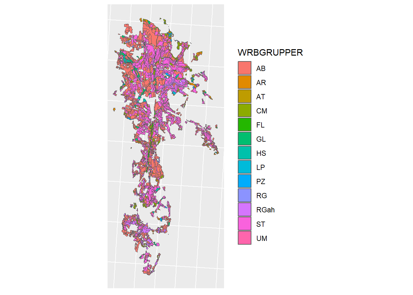

Figure 1.6: Jordsmonn Map for CS10

It only covers agricultural land, and therefore is not enough for complete coverage of the catchment, for this we need to combine it with our with out other map, Loesmasser.

lm_path <- "model_data/input/soil/loesmasser_cs10.shp"
lm_shp <- read_sf(lm_path)
lm_plot <- ggplot(lm_shp) + geom_sf(mapping = aes(fill = jorda_navn)) + sf_theme
lm_plot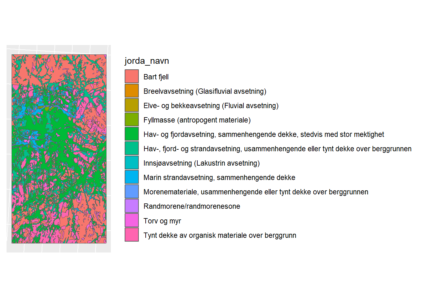

Figure 1.7: Loesmasser Map for CS10

1.2.3 Combining Jordsmonn and Loesmasser

Are they in the same CRS?

st_crs(lm_shp) == st_crs(jm_shp)

## [1] TRUE

We will need a mask of the JM (unite it to a single polygon)

jm_mask <- st_union(jm_shp)

ggplot(jm_mask) + geom_sf(fill = "orange") + sf_theme

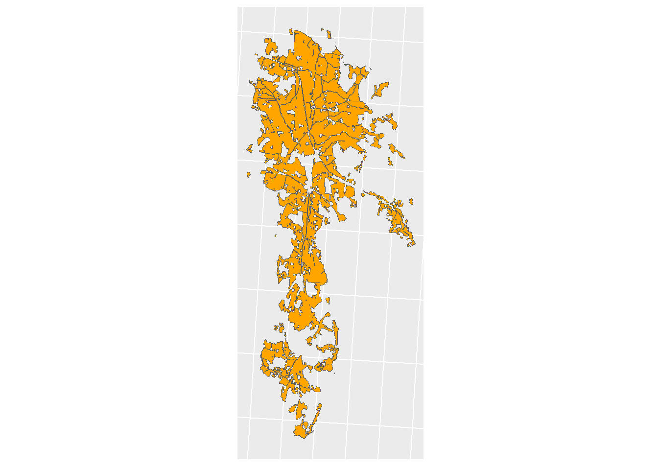
Figure 1.8: Jordsmonn Mask

And now we need to clip LM

clipped_lm <- st_difference(lm_shp, jm_mask)

## Warning: attribute variables are assumed to be spatially constant throughout
## all geometries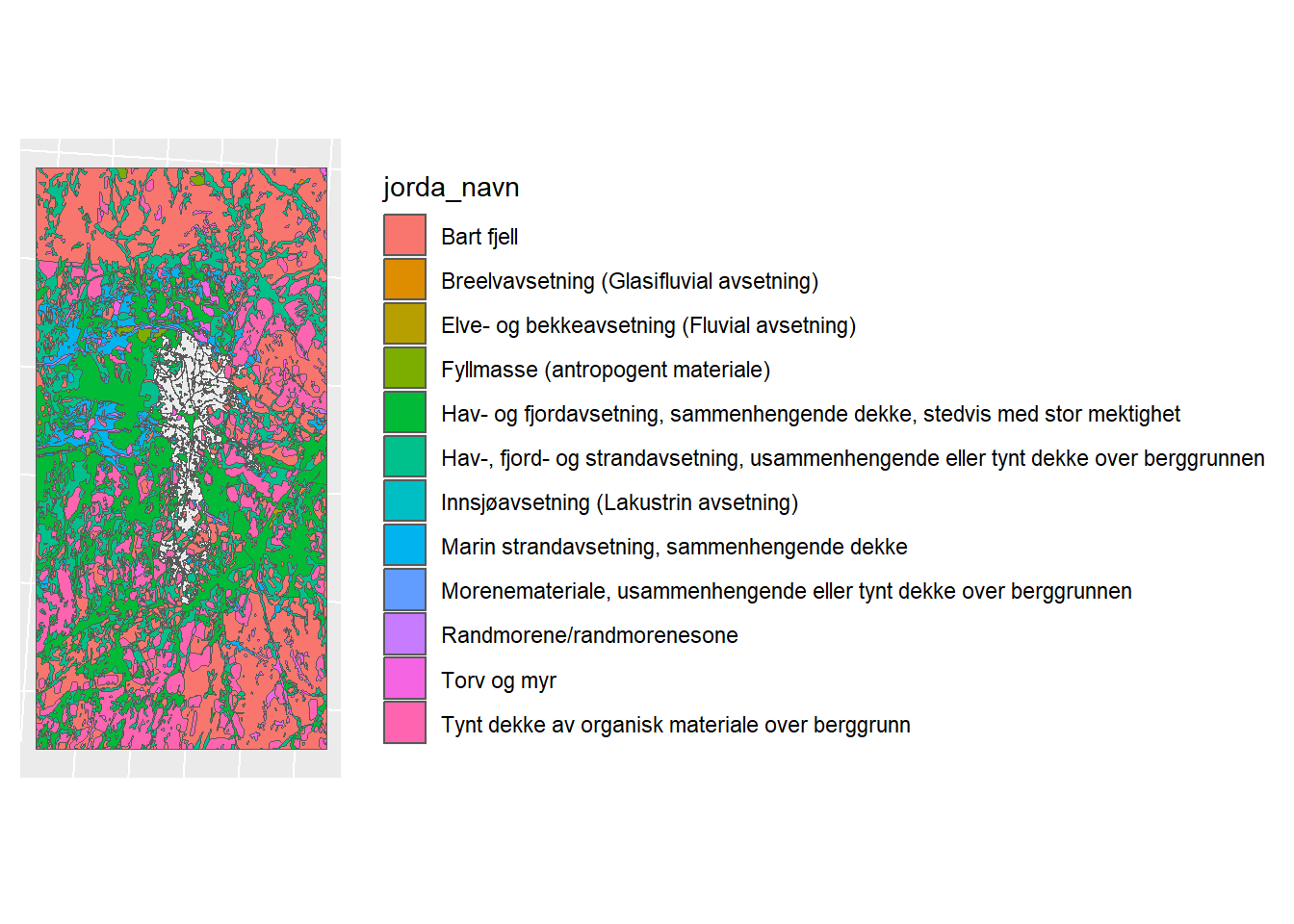

ggplot(clipped_lm) + geom_sf(mapping = aes(fill = jorda_navn)) + sf_theme

Figure 1.9: Clipped Loesmasser Map

Now we can merge the two maps. But the columns must match:

jm_shp_sel <- jm_shp %>% dplyr::select(geometry, WRBGRUPPER)
lm_shp_sel <- clipped_lm %>% dplyr::select(geometry, jorda_navn)
colnames(jm_shp_sel) <- c("geometry", "name")
colnames(lm_shp_sel) <- c("geometry", "name")

Merge the names

soil_union <- rbind(jm_shp_sel, lm_shp_sel)

Rename the absurdly long soil names:

soil_union$name <- soil_union$name %>%
  str_replace("Hav-, fjord- og strandavsetning, usammenhengende eller tynt dekke over berggrunnen", "Sea_dep_thin") %>% 
  
  str_replace("Hav- og fjordavsetning, sammenhengende dekke, stedvis med stor mektighet", "Sea_dep_thick") %>% 
  
  str_replace("Marin strandavsetning, sammenhengende dekke", "Beach_dep") %>% 
  
  str_replace("Tynt dekke av organisk materiale over berggrunn", "Humic") %>% 
  
  str_replace("Randmorene/randmorenesone", "End_moraine") %>% 
  
  str_replace("Bart fjell", "Mountain") %>% 
  
  str_replace("Torv og myr", "Bog_organic") %>% 
  
  str_replace("Morenemateriale, usammenhengende eller tynt dekke over berggrunnen", "moraine_dep")

soil_union$name[which(soil_union$name == "Fyllmasse (antropogent materiale)")] = "Antropogenic"

soil_union$name[which(soil_union$name == "Elve- og bekkeavsetning (Fluvial avsetning)")] = "river_dep"

soil_union$name[which(soil_union$name == "Innsjøavsetning (Lakustrin avsetning)")] = "lake_dep"

soil_union$name[which(soil_union$name == "Breelvavsetning (Glasifluvial avsetning)")] = "glacier_dep"

The map:

ggplot(soil_union) + geom_sf(mapping = aes(fill = name)) + sf_theme

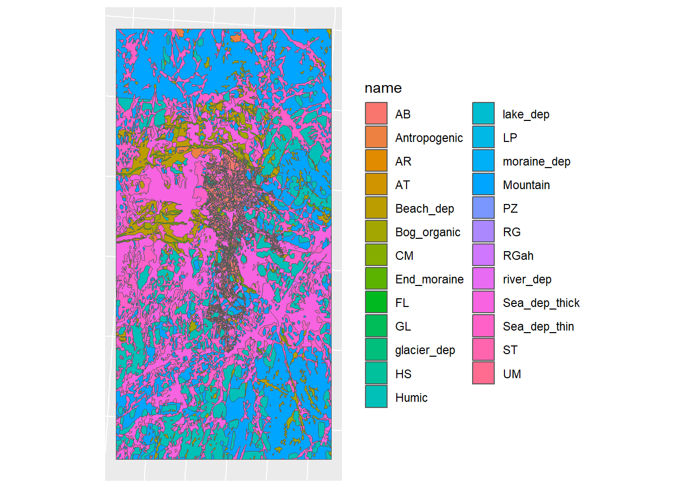
Figure 1.10: Merged soil map for CS10

Now we need to relate these classes to those we have in the soil data, which is located here:

usersoil <- read_csv("model_data/input/soil/usersoil_26.csv", show_col_types = F)

And contains these soil names:

usersoil$SNAM %>% unique() %>% sort()

##  [1] "ANT" "ARD" "BEA" "BOG" "CMD" "CME" "END" "GLC" "GLU" "HS"  "HUM" "LV" 
## [13] "MON" "PL"  "PZ"  "RG"  "SDD" "SDS" "STC" "STE" "STL" "STP" "STR" "STS"
## [25] "STV" "TUM"

These are 26 soil classes

usersoil$SNAM %>% unique() %>% length()

## [1] 26

Which is more than our soil map has

soil_union$name %>% unique() %>% length()

## [1] 25

Therefore, this Jordmonn map is not detailed enough for our desired 26 soil classes.

1.2.4 Detailed Soil Map

Thankfully we have a more detailed map which contains more information from NIBIOs internal maps department. This is located here:

jm_detailed <- "model_data/input/soil/soil_map_detailed.shp"
jm_detailed_shp <- read_sf(jm_detailed)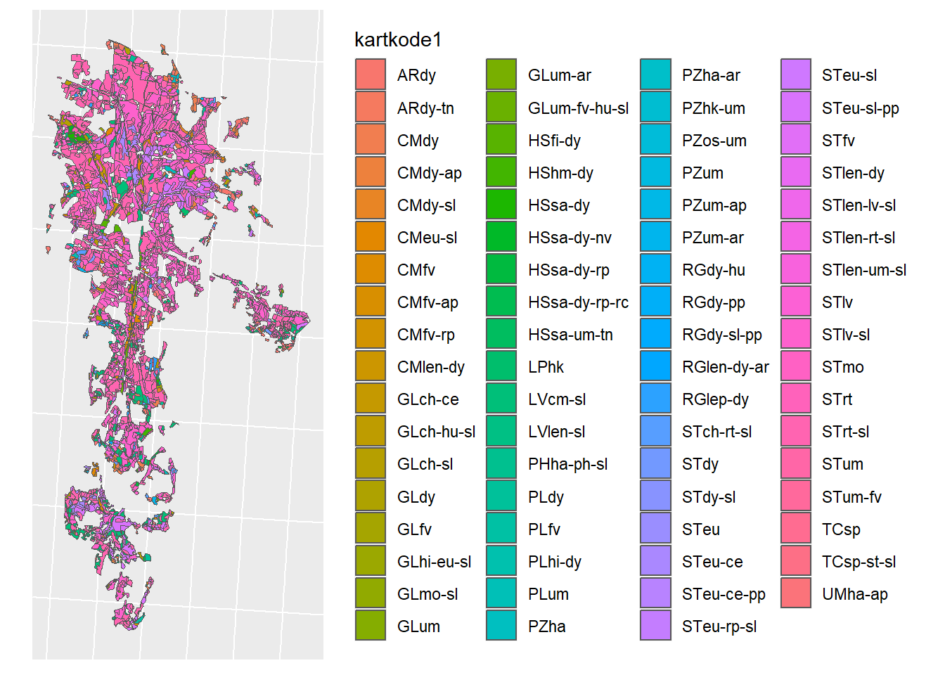

ggplot(jm_detailed_shp) + geom_sf(mapping = aes(fill = kartkode1)) + sf_theme

Figure 1.11: Detailed soil map for CS10 from the NIBIO maps department.

That is way more.

Same CRS?

st_crs(jm_detailed_shp) == st_crs(lm_shp)

## [1] TRUE

We will now repeat the process with the detailed map:

jm_det_mask <- st_union(jm_detailed_shp)
clipped_lm <- st_difference(lm_shp, jm_det_mask)

## Warning: attribute variables are assumed to be spatially constant throughout
## all geometries

jm_shp_sel <- jm_detailed_shp %>% dplyr::select(geometry, kartkode1)
lm_shp_sel <- clipped_lm %>% dplyr::select(geometry, jorda_navn)
colnames(jm_shp_sel) <- c("geometry", "name")
colnames(lm_shp_sel) <- c("geometry", "name")
soil_union <- rbind(jm_shp_sel, lm_shp_sel)

jm_det_select <- jm_detailed_shp %>% dplyr::select(geometry, kartkode1)
colnames(jm_det_select) <- c("geometry", "name")

soil_union_det <- rbind(jm_det_select, lm_shp_sel)

soil_union_det$name <- soil_union_det$name %>%
  str_replace("Hav-, fjord- og strandavsetning, usammenhengende eller tynt dekke over berggrunnen", "Sea_dep_thin") %>% 
  
  str_replace("Hav- og fjordavsetning, sammenhengende dekke, stedvis med stor mektighet", "Sea_dep_thick") %>% 
  
  str_replace("Marin strandavsetning, sammenhengende dekke", "Beach_dep") %>% 
  
  str_replace("Tynt dekke av organisk materiale over berggrunn", "Humic") %>% 
  
  str_replace("Randmorene/randmorenesone", "End_moraine") %>% 
  
  str_replace("Bart fjell", "Mountain") %>% 
  
  str_replace("Torv og myr", "Bog_organic") %>% 

  str_replace("Morenemateriale, usammenhengende eller tynt dekke over berggrunnen", "End_moraine")

### This will be simplified right now:
soil_union_det$name[which(soil_union_det$name == "Fyllmasse (antropogent materiale)")] = "Antropogenic"
soil_union_det$name[which(soil_union_det$name == "Breelvavsetning (Glasifluvial avsetning)")] = "End_moraine"
soil_union_det$name[which(soil_union_det$name == "Innsjøavsetning (Lakustrin avsetning)")] = "Sea_dep_thick"
soil_union_det$name[which(soil_union_det$name == "Elve- og bekkeavsetning (Fluvial avsetning)")] = "Sea_dep_thick"

We now have 79 soil classes.

soil_union_det$name %>% unique() %>% length()

## [1] 79

We will save this because it will come in handy later

sf::write_sf(soil_union_det, "model_data/input/soil/soil_map_79.shp")

1.2.5 Reclassification

We will rename and simplify the classes like so:

soil_reclass <- read_csv("model_data/input/soil/soil_reclass.csv",show_col_types = F)
datatable(soil_reclass)

Reclassification Loop

soil_union_det$id = NA
for (soil in soil_reclass$old_name) {
  reclassed <- soil_reclass$new_name[which(soil_reclass$old_name == soil)]
  ID <- soil_reclass$id[which(soil_reclass$old_name == soil)]
  soil_union_det$name[which(soil_union_det$name == soil)] <- reclassed
  soil_union_det$id[which(soil_union_det$name == soil)] <- ID
}

Now let us map it:

soil_complex_plot <- ggplot(soil_union_det) + geom_sf(mapping = aes(fill = name)) + sf_theme
soil_complex_plot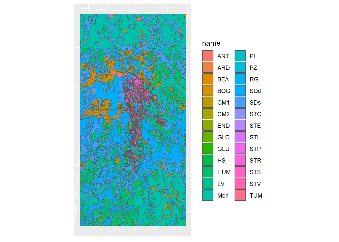

Figure 1.12: Reclassified detailed map

1.2.6 Simplifying Geometries

We can simplify the geometry by aggregating by soil name

soil_simple <- soil_union_det %>% group_by(name) %>% summarize()

soil_simple_plot <- ggplot(soil_simple) + geom_sf(mapping = aes(fill = name)) + sf_theme
soil_simple_plot

Figure 1.13: Simplified Geometry of the soil map

And a comparison:

Figure 1.14: Soil map simplification

1.2.7 Writing vector layer

We will need this vector layer later on in the project, so we will save it now

sf::write_sf(soil_simple, "model_data/input/soil/cs10_soil_map.shp")

1.2.8 Lookup Table

In its final form, this map needs to be a RASTER with the ID as a value, and we need a lookup table to relate the ID to the soil.

Creating the look-up table

new_name <- soil_reclass %>% dplyr::select(new_name) %>% dplyr::pull() %>% base::unique()
soil_lookup <- data.frame(SOIL_ID = seq_along(new_name), SNAM = new_name)
write_csv(x = soil_lookup, file = "model_data/input/soil/soil_lookup_26.csv")

1.2.9 Rasterization

We need to relate these new IDs to our soil map with a left join

soil_simple$SNAM <- soil_simple$name
soil_simple_id <- left_join(x = soil_simple, y = soil_lookup, by = "SNAM")
ggplot(soil_simple_id) + geom_sf(mapping = aes(fill = SOIL_ID)) + sf_theme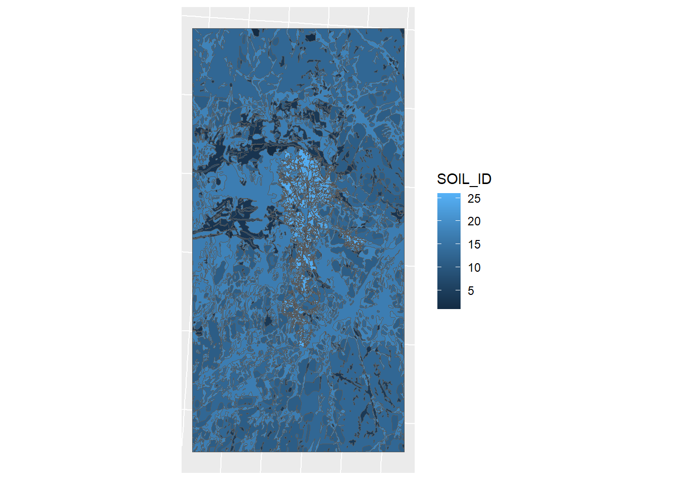

Figure 1.15: Soil map by soil ID

Now we need to rasterize with this ID as the value.

soil_rast <-
  stars::st_rasterize(soil_simple_id,
              stars::st_as_stars(sf::st_bbox(soil_simple_id),
                          nx = 3060, # resolution matches the original
                          ny = 5352) # resolution marches the original
              )
soil_rast <- as(soil_rast, "SpatRaster") 

plot(soil_rast)

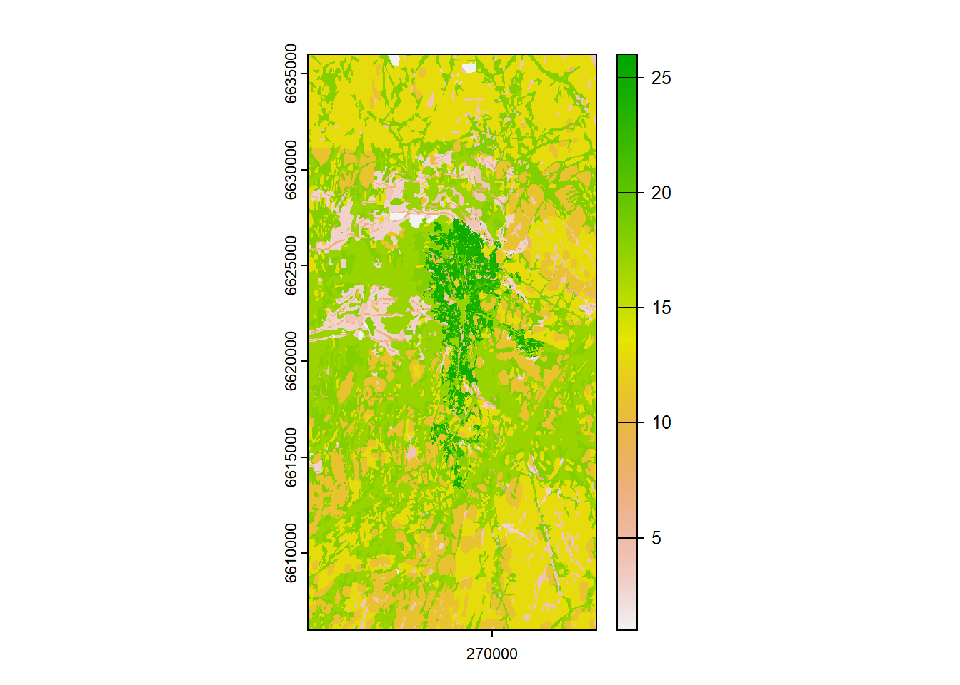
Figure 1.16: Rasterized soil map

Check the values:

# crop to watershed extent
wsmask <- soil_rast %>% 
  terra::crop(., read_sf("model_data/input/shape/cs10_basin_1m.shp"))
# get frequency of pixels
soil_histogram <- raster::freq(wsmask)
# convert to tibble
soil_hist <- as_tibble(soil_histogram)
# get total sum for relative value
total_pixels <- soil_hist$count %>% sum()
# relative value calculation
soil_hist$rel <- (soil_hist$count/total_pixels)*100
# Round to 2 decimals
soil_hist$rel<-soil_hist$rel %>% round(2)
# left join look up table
soil_hist$SOIL_ID <- soil_hist$value
soil_hist <- left_join(soil_hist, soil_lookup, by = "SOIL_ID")
# sort by size
soil_hist<-soil_hist %>% arrange(rel)
# Rearrange and drop duplicate columns
soil_hist <- soil_hist %>% dplyr::select(SOIL_ID, SNAM, count, rel)

datatable(soil_hist)

Pie chart of results:

# Get the positions
df2 <- soil_hist %>% 
  mutate(csum = rev(cumsum(rev(rel))), 
         pos = rel/2 + lead(csum, 1),
         pos = if_else(is.na(pos), rel/2, pos))
# Pie chart
ggplot(soil_hist, aes(x = "" , y = rel, fill = reorder(SNAM, rel))) +
  geom_col(width = 1, color = 1) +
  coord_polar(theta = "y") +
  geom_label_repel(
    data = df2,
    aes(y = pos, label = paste0(SNAM, " ", rel, "%")),
    size = 2,
    force = 3,
    nudge_x = 1,
    show.legend = FALSE,
    box.padding = 0,
    seed = 123456,
    force_pull = 0,
    direction = "both",
    max.overlaps = 26
  ) +
  guides(fill = guide_legend(title = "Soil")) +
  theme_void()

Figure 1.17: Soil distribtution within the catchment area.

And check the CRS

print(soil_rast)

## class       : SpatRaster 
## dimensions  : 5352, 3060, 1  (nrow, ncol, nlyr)
## resolution  : 4.905229, 5.60725  (x, y)
## extent      : 260425, 275435, 6605995, 6636005  (xmin, xmax, ymin, ymax)
## coord. ref. : ETRS89 / UTM zone 33N (EPSG:25833) 
## source(s)   : memory
## name        : SOIL_ID 
## min value   :       1 
## max value   :      26

raster::writeRaster(soil_rast, "model_data/input/soil/soil_raster.tif", overwrite = T)

1.2.10 Usersoil

We need to update our usersoil data now to match the IDs, as we can see there are quite a few differences:

usersoil26 <- read_csv("model_data/input/soil/usersoil_26.csv", show_col_types = F)
US <- usersoil26 %>% select(OBJECTID, SNAM)
US <- US %>% arrange(SNAM)
compare <- cbind(US, soil_lookup %>% arrange(SNAM))
datatable(compare)

A few names are mismatched as well

usersoil26$SNAM[which(usersoil26$SNAM == "CMD")] = "CM1"
usersoil26$SNAM[which(usersoil26$SNAM == "CME")] = "CM2"
usersoil26$SNAM[which(usersoil26$SNAM == "SDS")] = "SDs"
usersoil26$SNAM[which(usersoil26$SNAM == "SDD")] = "SDd"
usersoil26$SNAM[which(usersoil26$SNAM == "MON")] = "Mon"

Reclassification loop:

for (soil in soil_lookup$SNAM) {
  new_id <- soil_lookup %>% filter(SNAM == soil) %>% select(SOIL_ID) %>% pull()
  old_id <- which(usersoil26$SNAM==soil)
  usersoil26$OBJECTID[old_id] = new_id
}

usersoil26$OBJECTID

##  [1]  2 13  5  6  1  8  9 18 17 10 11 12  3 14 15  7 16 19 20 21 22 23 24 25  4
## [26] 26

Lets sort by the new order.

usersoil_ordered <- usersoil26[order(usersoil26$OBJECTID),]

Now we can write the changes with the updated IDs

write_csv(usersoil_ordered, "model_data/input/soil/usersoil_26_v2.csv")

1.3 Watershed Boundary

The watershed boundary must be a single polygon GIS vector layer. Presumed source of the data is NVE. It is located here:

basin_path <- "model_data/input/shape/cs10_basin.shp"

We will be following this guide to create it using whitebox tools (REF).

We will be using a single tile of our 1 DEM to start, since the whole dataset is large

dem <- raster("model_data/input/elevation/cs10_dem_1m_utm33n.tif")

plot(dem, main = "UTM 33N")

1.3.1 Hydrological preperation

Time to breach and fill:

wbt_breach_depressions_least_cost(
  dem = "model_data/input/elevation/cs10_dem_1m_utm33n.tif",
  output = "model_data/input/elevation/intermediates/dem_breached.tif",
  dist = 5,
  fill = TRUE)

wbt_fill_depressions_wang_and_liu(
  dem = "model_data/input/elevation/intermediates/dem_breached.tif",
  output = "model_data/input/elevation/intermediates/dem_filled_breached.tif"
)

Flow Accumulation

wbt_d8_flow_accumulation(input = "model_data/input/elevation/intermediates/dem_filled_breached.tif",
                         output = "model_data/input/elevation/intermediates/D8FA.tif")

And D8 pointer

wbt_d8_pointer(dem = "model_data/input/elevation/intermediates/dem_filled_breached.tif",
               output = "model_data/input/elevation/intermediates/D8pointer.tif")

1.3.2 Pour Points

Our outlet point is located here:

outlet <- "model_data/input/point/cs10_outlet_utm33n.shp"
outlet_point <- read_sf(outlet)
outlet_map <- mapview(outlet_point)
outlet_map

We will need to snap it to the channel network. But first we need those streams.

1.3.3 Streams

Extracting our streams

wbt_extract_streams(flow_accum = "model_data/input/elevation/intermediates/D8FA.tif",
                    output = "model_data/input/elevation/intermediates/raster_streams.tif",
                    threshold = 6000)

To verify this threshold, lets have a look at the map

stream_rast <- rast("model_data/input/elevation/intermediates/raster_streams.tif")

plot(stream_rast)

That does not look good. But if we zoom in:

plot(stream_rast, xlim = c(269400,269500), ylim = c(6622100, 6622200))

Lets check if they line up with our actual streams.

extent_coord <- data.frame(
  Plot = c("A", "A", "A", "A"),
  Corner = c("SW", "NW", "NE", "SE"),
  
  Easting = c(268280,  # SW
              268280,  # NW
              268480,  # NE
              268480), # SE
  
  Northing = c(6613423, # SW
               6613623, # NW
               6613623, # NE
               6613423) # SE
  )
  
  extent <- sfheaders::sf_polygon(
  obj = extent_coord
  , x = "Easting"
  , y = "Northing"
  , polygon_id = "Plot"
)
  
  sf::st_crs(extent) <- 25833

  mapview(extent)+outlet_map

Cropping by our extent, and checking the location of the pixels referenced to a map:

stream_crop <- raster::crop(stream_rast, extent)
stream_crop <- as(stream_crop, "Raster")
stream_crop_map <- mapview(stream_crop, maxpixels =  2200000)
stream_crop_map

Looks good.

Snapping our pour point to the network

wbt_jenson_snap_pour_points(
  pour_pts = "model_data/input/point/cs10_outlet_utm33n.shp",
  streams = "model_data/input/elevation/intermediates/raster_streams.tif",
  output = "model_data/input/point/snappedpp.shp",
  snap_dist = 35) #careful with this! Know the units of your data

Did it work?

pp <- shapefile("model_data/input/point/snappedpp.shp")
streams <- raster("model_data/input/elevation/intermediates/raster_streams.tif")

stream_crop_map+mapview(pp)

It seems to have worked.

1.3.4 Watershed Delineation

Finally, we are ready to delineate the watershed.

wbt_watershed(d8_pntr = "model_data/input/elevation/intermediates/D8pointer.tif",
              pour_pts = "model_data/input/point/snappedpp.shp",
              output = "model_data/input/elevation/intermediates/dem_basin.tif")

Preview:

ws <- raster::raster("model_data/input/elevation/intermediates/dem_basin.tif")
mapview(ws)

## Warning in rasterCheckSize(x, maxpixels = maxpixels): maximum number of pixels for Raster* viewing is 5e+05 ; 
## the supplied Raster* has 450450100 
##  ... decreasing Raster* resolution to 5e+05 pixels
##  to view full resolution set 'maxpixels =  450450100 '

Now we need this in polygon form.

wsshape <- stars::st_as_stars(ws) %>% sf::st_as_sf(merge = T)

ws_1m_map <- mapview(wsshape)
ws_1m_map

Amazing, so high res.

Lets write it

sf::write_sf(wsshape, "model_data/input/shape/cs10_basin_1m.shp")

A comparison to the old 10m dem:

dem10m <- read_sf("model_data/input/shape/cs10_basin.shp")
ws_1m_map+mapview(dem10m, col.region = "orange")

1.3.5 Bonus Section

Lets make a 3D map for fun

dem <- raster::raster("model_data/input/elevation/cs10_dem_1m_utm33n.tif")

#crop
wsmask <- dem %>%
  terra::crop(.,extent ) %>%
  terra::mask(., extent)

#convert to matrix
wsmat <- matrix(
  terra::extract(wsmask, extent(wsmask)),
  nrow = ncol(wsmask),
  ncol = nrow(wsmask))

#create hillshade
raymat <- ray_shade(wsmat, sunangle = 115)

#render
wsmat %>%
  sphere_shade(texture = "desert") %>%
   add_water(detect_water(wsmat), color = "desert") %>%
  #add_shadow(raymat) %>%
  plot_3d(
    wsmat,
    zscale = .8,
    fov = 0,
    theta = 135,
    zoom = 0.75,
    phi = 45,
    windowsize = c(750, 750)
  )
rglwidget()

1.4 Land object input

Requirements:

1. column id number for each element
2. column type defining land use
3. column drainage containing the id of the channel receiving water from the drained field.

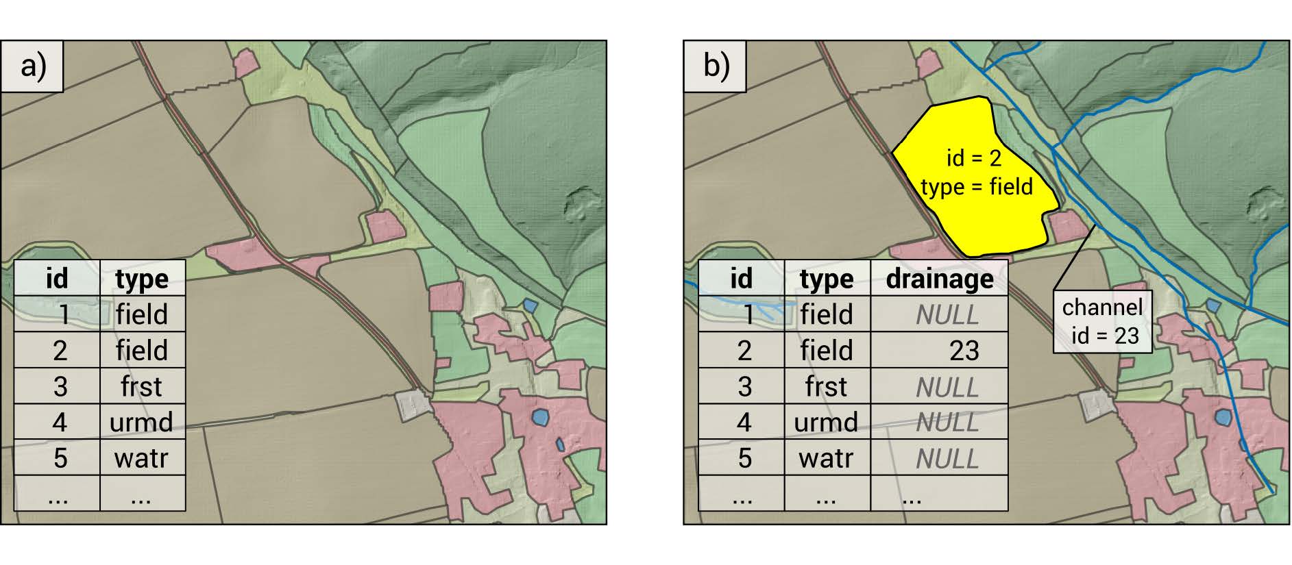
Figure 1.18: Land object polygons with attribute table. a) shows a land layer without tile drainage implemented. b) shows a case where the agricultural field with the land id = 2 has tile drainage activated and drains the tile flow into the channel id = 23 Schürz et al. (2022)

The creation of the land object map was not documented. It is located here:

lo_path <- "model_data/input/land/CS10_LU.shp"

A preview:

lo_shp <- read_sf(lo_path)
lo_plot <- ggplot(lo_shp) + geom_sf(mapping = aes(fill = drainage)) + sf_theme +
  ggtitle("CS10 Landuse map", "Tile drainage indicated by ID of recieving channel")
print(lo_plot)

Figure 1.19: CS10 Landuse map

1.4.1 Data sources

Only partial documentation is available:

1. For Landuse, the Corine landcover 2018 (CLC) sourced from NIBIOs map service kart8 (details unknown)

2. Field boundaries were sourced from the norwegian property register, hosted on kartverket (details unknown)

1.4.2 Delineation of land objects

Currently not documented

1.4.3 Standing water bodies and the landuse type = ‘watr’

Currently not documented

1.4.4 Tile drainage option

To determine which of our agricultural fields need drainage, we are going to use the Jordsmonn Map, specifically the Natural drainage capacity (Naturlige dreneringsforhold) described in column “JR_DREN”. Documentation for this dataset can be found here. The datasets have been clipped to the catchment area before this analysis (to reduce file sizes and computation time).

Discussion of this topic can be found in Issue #65

jordmonn <- "model_data/input/soil/jordsmonn.shp"
jm_shp <- read_sf(jordmonn)

There is a lot of junk in this file (89 columns of data), we only need JR_DREN

jm_shp_filt <- jm_shp %>% select(geometry, JR_DREN)

Classes 1,2 and 3 have the need for tile drains, whereas class 4 has enough natural drainage capacity to forgo tile drainage.

jm_drained <- jm_shp_filt %>% filter(JR_DREN != "4")
jm_not_drained <- jm_shp_filt %>% filter(JR_DREN == "4")

A comparison:

Figure 1.20: Tile drainage Classes

The drainage column of our land use map has already been defined, however every field regardless of its natural drainage class, has been assigned tile drains. We will now remove the tile drains which are located on class 4 soils.

First we will drop any unneeded data in our cluttered land object map.

lu_map <- lo_shp %>% select(geometry, id, type, drainage)

And convert our drainage map to the same projection.

jm_shp_filt <- st_transform(jm_shp_filt, st_crs(lu_map))

Then we will join the drainage class attribute spatially.

intersect_pct_4 <- st_intersection(lu_map, jm_shp_filt %>% filter(JR_DREN == "4")) %>% 
   mutate(intersect_4 = st_area(.)) %>%   # create new column with shape area
   dplyr::select(id, intersect_4) %>%   # only select columns needed to merge
   st_drop_geometry() 

## Warning: attribute variables are assumed to be spatially constant throughout
## all geometries

intersect_pct_not_4 <- st_intersection(lu_map, jm_shp_filt %>% filter(JR_DREN != "4")) %>% 
   mutate(not_4 = st_area(.)) %>%   # create new column with shape area
   dplyr::select(id, not_4) %>%   # only select columns needed to merge
   st_drop_geometry() 

## Warning: attribute variables are assumed to be spatially constant throughout
## all geometries

Total the individual intersectoins

class_4 <- intersect_pct_4 %>% group_by(id) %>% summarise(class_4 = sum(intersect_4))
not_class_4 <- intersect_pct_not_4 %>% group_by(id) %>% summarise(not_class_4 = sum(not_4))

Left join them to our land use map by their ID

lu_drains <- left_join(lu_map, class_4, by = "id")
lu_drains <- left_join(lu_drains, not_class_4, by = "id")

Set NA values to 0

lu_drains$class_4[which(lu_drains$class_4 %>% is.na())] = 0
lu_drains$not_class_4[which(lu_drains$not_class_4 %>% is.na())] = 0

Predefining our natural drainage attribute as false and defining our generic land use classes which are to be excluded from the manipulation.

lu_drains$natural_drain = FALSE
generics <- c("frst","rngb","urml","utrn","past", "watr", "wetf")

lu_drains$natural_drain[which((lu_drains$class_4 >= lu_drains$not_class_4) &
                           (lu_drains$type %in% generics == FALSE))] = TRUE

How many drains are we removing?

removed_len <- which((lu_drains$class_4 >= lu_drains$not_class_4) & 
                       (lu_drains$type %in% generics == FALSE)) %>% length()
removed_len

## [1] 238

Seems like a lot, but how many drained HRUs are there in total?

total_drains <- lu_map %>% filter(drainage > 0) %>% pull(drainage) %>% length()
total_drains

## [1] 1947

paste(((removed_len / total_drains) * 100) %>% round(1),
      "% of drained agricultural HRUs will have their drains removed.")

## [1] "12.2 % of drained agricultural HRUs will have their drains removed."

Time to remove:

lu_drains$drainage[which(lu_drains$natural_drain == TRUE)] = NA

And drop the columns we don’t need

lu_map_v2 <- lu_drains %>% select(geometry, id, type, drainage)

Which fields are naturally drained?

basin_map + mapview(lu_drains %>% filter(natural_drain), zcol = "type", legend = FALSE)

Our land use map now looks like this. The Number value points to the channel being drained to.

lu_v2 <-
  ggplot(lu_map_v2) + geom_sf(mapping = aes(fill = drainage)) + sf_theme +
  ggtitle("CS10 Landuse map",
          "Tile drainage indicated by ID of recieving channel")

print(lo_plot)

print(lu_v2)

Figure 1.21: Tile drainage which was removed

Time to save the changes:

write_sf(lu_map_v2, "model_data/input/land/CS10_LU_V2.shp")

And cleanup

rm(list = ls())

1.4.5 Existing and potential structures to retain water and nutrients

Currently not documented

1.5 Channel object input

Limited documentation available:

Stream-Reach vector was created using QSWAT

1.5.1 Data sources and data processing

Currently not documented

1.6 Point sources locations

BuildR can automatically add point source data if it is in the correct format and location. The requirements are as follows:

1. Same folder as point source location layer (shapefile)

And

2. the files must be named as <name>_<interval>.csv, where <name> must be the name of a point int the vector layer and <interval> must be one of const, yr, mon, or day depending on the time intervals in the input data.

This second point makes little sense but we will try out best.

1.6.1 Point source source data

ps <- readr::read_csv("model_data/input/pointsource/pointsourcedata.csv",
                            show_col_types = F)

# Select the columns we need
ps2 <- ps %>% dplyr::select(ID, x, y, tot_P_kg_a)

We have a problem. SWAT needs these data in terms of KG / m3 of outflow. We do not have outflow and just have total values. Therefore we need some sort of average outflow to divide our yearly total with.

ps2$flo = 1
# TODO

# Add columns for data we might add down the line
ps2$sed = NA
ps2$orgn = NA
ps2$sedp = ps2$tot_P_kg_a
ps2$no3 = NA
ps2$solp = NA
ps2$chla = NA
ps2$nh3 = NA
ps2$no2 = NA
ps2$cbod = NA
ps2$dox = NA
ps2$sand = NA
ps2$silt = NA
ps2$clay = NA
ps2$sag = NA
ps2$lag = NA
ps2$gravel = NA
ps2$tmp = NA

# drop the original P column
ps2 <- ps2 %>% dplyr::select(!tot_P_kg_a)

Our IDs are not unique

ps2$ID %>% length()

## [1] 5459

Why? We do not know. No metadata was provided with the file.

ps2$ID %>% unique() %>% length()

## [1] 1362

However every coordinate pair is unique

paste(ps2$x, ps2$y) %>% unique() %>% length()

## [1] 5429

We will need new IDs, but only for the ones in the catchment:

# creating a shape file from the coordinates (UTM32N) and transforming to UTM33N
point_source_shape <- ps2 %>% 
  sf::st_as_sf( coords = c("y", "x") ) %>%
  sf::st_set_crs(25832) #%>%  # UTM 32N
  #sf::st_transform(25833) # UTM 33N

# Cropping to DEM extent

basin_shp <- read_sf("model_data/input/shape/cs10_basin.shp")# %>% sf::st_transform(25833)
point_source_shape_crop <- point_source_shape %>% 
  sf::st_intersection(., basin_shp)

point_source_shape_crop$name <- paste0("pssite_", seq_along(point_source_shape_crop$ID))


# Write the shape file
sf::write_sf(obj = point_source_shape_crop,
          dsn = "model_data/input/pointsource/cs10-ps-data.shp")

1.6.2 Point source data files

We need to create .csv files in the same directory which contain the point source values.

psdata <- point_source_shape_crop %>% st_drop_geometry() %>% dplyr::select(name, flo, sedp)
for (i in seq_along(psdata$name)) {
  line <- psdata[i,] %>% select(-name)
  file_path = paste0("model_data/input/pointsource/",psdata$name[i],"_const.csv")
  write.table(x = line,
              file_path,
              row.names = F,
              col.names = T,
              quote = F, sep = ",")
}

1.7 Aquifer Objects

Aquifers are not an important part of the OPTAIN setup, no work needs to be done here:

Although SWAT+ would allow the implementation of multiple aquifers in a model setup, the current version of SWATbuildR only adds a single aquifer for the entire catchment to the model setup. All land and water objects will be linked to this single aquifer. As the sizes of the OPTAIN study sites range between approximately 20 to 250 km2 the use of a single aquifer can be justified.

References

Schürz, Christoph, Natalja Čerkasova, Csilla Farkas, Attila Nemes, Plunge, Michael Strauch, Brigitta Szabó, and Mikołaj Piniewski. 2022. “SWAT+ Modeling Protocol for the Assessment of Water and Nutrient Retention Measures in Small Agricultural Catchments,” December. https://doi.org/10.5281/ZENODO.7463395.