Section 5 Crop Map Generation
As OPTAIN takes into account the individual field, we need to know what is growing on which field and when. Unfortunately our data foundation for this task is quite lackluster, but we will try out best to do so. in the following chapter.
require(sf)
require(dplyr)
require(readr)
require(stringr)
require(readxl)
require(reshape2)
require(tibble)
require(DT)
require(ggplot2)
require(gifski)

sf_theme <- theme(axis.text.x=element_blank(), #remove x axis labels
        axis.ticks.x=element_blank(), #remove x axis ticks
        axis.text.y=element_blank(),  #remove y axis labels
        axis.ticks.y=element_blank()  #remove y axis ticks
        )
5.1 Calculating Field Area
We have data based on what area certain crops have per farm. In order to relate this to our spatial land use map, we require the area of both the farms, and the fields within these farms.
The basis for these calculations comes from the BuildR output from Section
lu_sf <- read_sf("model_data/cs10_setup/optain-cs10/data/vector/land.shp")
lu_map <- ggplot() + geom_sf(lu_sf, mapping = aes(fill = type)) +
  theme(legend.position = "left") + sf_theme + theme(legend.position = "none")
print(lu_map)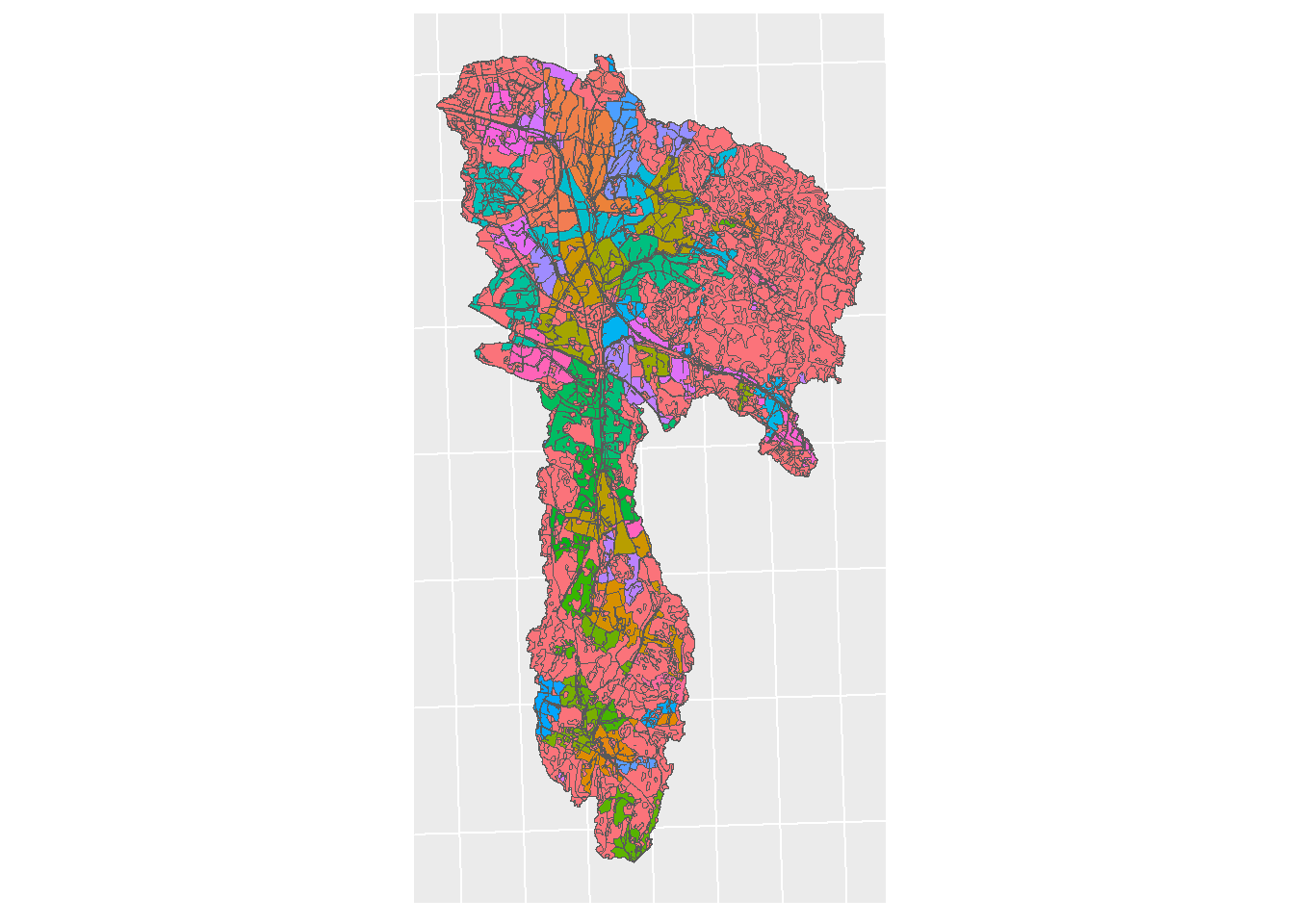
Figure 5.1: Land use map for CS10, colored by type.
5.1.1 Calculate Field Area and Assign IDs
This stage has been completed in QGIS. An R-implementation is being considered.
farm_area_sf <-
  read_sf("model_data/input/crop/buildr_output_dissolved_into_farms.shp")
field_lu_plot <-
  ggplot() + geom_sf(farm_area_sf, mapping = aes(fill = farm_id)) +
  theme(legend.position = "none") + sf_theme
print(field_lu_plot)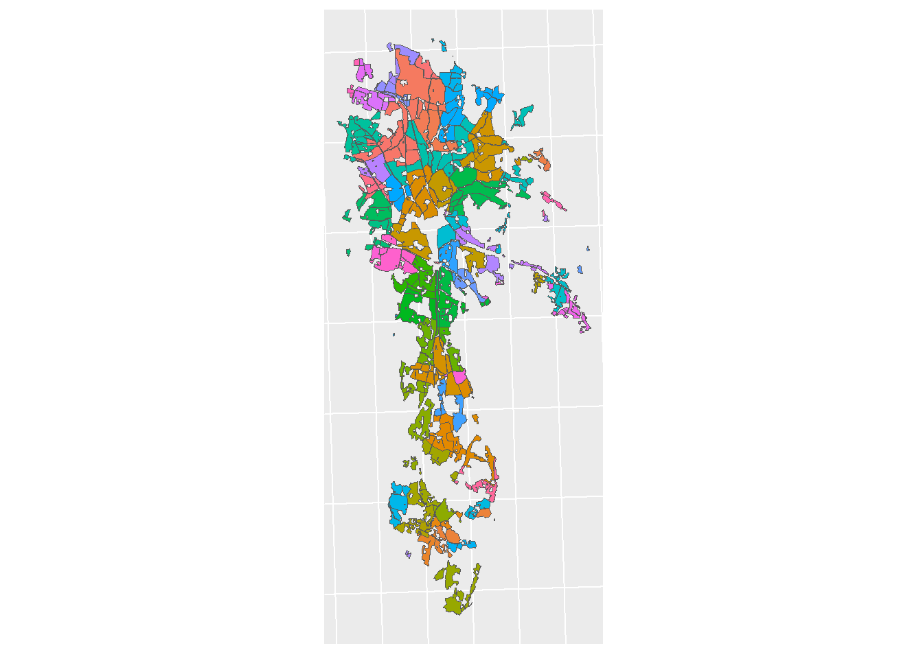
Figure 5.2: Farms in the CS10 catchment, colored by ID
5.2 Generating the Crop Rotation
The following algorithm takes information from reporting farm, and their respective area in the SWAT+ setup, and combines these data sets to generate a plausible crop rotation.
Note, pasture refers to meadow (TODO: fix!)
crop_data <- read_excel("model_data/input/crop/crop_rotation_source_data.xlsx")
datatable(crop_data)
5.2.1 Tidy up the source data:
We are converting the source data to tidy format in the following code snippet
 crop_names <- melt(
    crop_data,
    id.vars = c("farm_id", "year", "area_daa", "pastrure_area_daa"),
    measure.vars = c("crop1", "crop2", "crop3"),
    variable.name = "crop_status", value.name = "crop"
  ) %>% tibble()
  crop_area <- melt(
    crop_data,
    id.vars = c("farm_id", "year", "area_daa", "pastrure_area_daa"),
    measure.vars = c("percent_crop1", "percent_crop2", "percent_crop3"),
    variable.name = "crop_status", value.name = "area"
  ) %>% tibble()
  crop_area$crop_status <- crop_area$crop_status %>% str_remove("percent_")
  # unstable, TODO fix!
  colnames(crop_area)[6] <- "crop_area_percent"
  crop_tidy <- left_join(crop_names, crop_area, by = c("farm_id", "year", "area_daa","pastrure_area_daa", "crop_status")) %>% dplyr::select(-crop_status)
   # unstable, TODO fix!
  colnames(crop_tidy)[3] <- "farm_area_daa"
  crop_tidy$crop_area_percent <- (crop_tidy$crop_area_percent/100) %>% round(2)
  crop_tidy <- crop_tidy %>% filter(crop %>% is.na() == FALSE)
  datatable(crop_tidy)
5.2.2 Tidy up the BuildR output
The maps shown in Section 5.1 were exported to CSV in QGIS. An R-implementation might be written in here sometime (#TODO).
This CSV data needs to be re-formatted to be tidy as well.
fields <-
  read_csv(
    "model_data/input/crop/buildr_landuse_dissolved_into_fields.csv",
    show_col_types = F
  ) %>% dplyr::select(type, farm_id, field_area_daa)

farms <-
  read_csv(
    "model_data/input/crop/buildr_landuse_dissolved_into_farms.csv",
    show_col_types = F
  ) %>% dplyr::select(type, farm_id , farm_area_)
# fix farm_area_ TODO
# unstable, fix! TODO
colnames(farms)[3] <- "farm_area_daa"
farms$farm_area_daa <- farms$farm_area_daa %>% round(2)
fields$field_area_daa <- fields$field_area_daa %>% round(2)
reported_data <- left_join(fields, farms, by = "farm_id")

# unstable, fix! TODO
colnames(reported_data)[1] <- "field_id"

reported_data <- reported_data %>% dplyr::select(field_id, farm_id, field_area_daa, farm_area_daa)

datatable(reported_data)
5.2.3 Field classification
We are now ready to perform our classification. We will store our results in this predefined dataframe:
classed_fields <-
  tibble(
    farm_id = NA,
    field_id   = NA,
    farm_area_daa = NA,
    field_area_daa = NA,
    crop  = NA,
    year = NA
  )
The following reporting farms will be used for the classification:
For the following years (AKA we have data for these years):
This for loop runs through all the fields and classifies them. The output will not be printed in this file, but will be saved in a log file, that you can dig out of the repository, located here:
The following code is not executed:
# For every year
for(c_year in years){
  # For every farm,
  for (farm in farms) {
    # Do the following:

    # Filter the source and buildR data to the given year and farm
    crop_filter <- crop_tidy %>% filter(year == c_year) %>% filter(farm_id == farm)
    hru_filter <- reported_data %>% filter(farm_id == farm)

    # Behavior if the farm has no reporting data:
    if(crop_filter$farm_id %>% length() == 0){

      # Set all fields to winter wheat.

      farm_fields <- hru_filter %>%
        dplyr::select(farm_id, field_id, farm_area_daa, field_area_daa) %>%
        arrange(desc(field_area_daa))

      farm_fields$crop = "wwht"
      farm_fields$year = c_year

      # Add them to the results dataframe
      classed_fields <- rbind(classed_fields, farm_fields)

      # and skipping to next farm
      next()
    }

    # Behavior, if there is reporting data on the farm"

    # Find the area of the farm (all elements in vector are the same, so ok
    # to just grab the first)
    farm_area_hru <- hru_filter$farm_area_daa[1]

    # Find the discrepency between "SHOULD BE" crop area and "CURRENTLY IS"
    # crop area. We want this as an absolute value.
    area_dis <- (hru_filter$farm_area_daa[1]-crop_filter$farm_area_daa[1]) %>%
      round(2) %>% abs()

    # Some farms have no reported area. in this case we set it to some random
    # negative number.
    if(area_dis %>% is.na()){area_dis = -999}

    # Extracting the area of the pasture and farm (all vectors same value, ok
    # to just take the first)
    past_area <- crop_filter$pastrure_area_daa[1]
    farm_area <- crop_filter$farm_area_daa[1]

    # Extract relevant fields
    farm_fields <- hru_filter %>%
      dplyr::select(farm_id, field_id, farm_area_daa, field_area_daa) %>%
      # and sort by area
      arrange(desc(field_area_daa))

    # pre-define crops column to be NA
    farm_fields$crop = NA

    # Bollean check to see if the field has been meadow in a previous year. If
    # it has, then we want to continue planting meadow on it (This was a
    # decision we made.)
    has_meadow <- (classed_fields %>% filter(field_id %in% farm_fields$field_id)
                   %>% filter(crop == "meadow") %>%
                     dplyr::select(field_id) %>% pull() %>% length() > 0)


    ### Determining how much land the crops should cover.

    # This if statement checks if is currently a pasture portion for the reporting
    # farm, or if there has been in the past.
    if((past_area %>% is.na() == FALSE) | has_meadow) {

      # If it does, or did, then this special routine is enacted:

      # Determines the pasture percentage of the total farm
      past_percent <- (past_area/farm_area)

      # If it cannot be calculated, then it is set to 0
      if(past_percent %>% is.na()){past_percent = 0}

      # The crop fractions provided to us in the source data did not account for
      # the pasture fraction. therefore we need to reduce the other crop
      # fractions by this amount.
      adjuster <- past_percent / length(crop_filter$crop)
      crop_filter$crop_area_percent <- crop_filter$crop_area_percent-adjuster

      # creating a new entry for pasture and adding it to the now updated crop\
      # fractions list
      past_row <-
        tibble(
          farm_id = farm,
          year = c_year,
          farm_area_daa = crop_filter$farm_area_daa[1],
          pastrure_area_daa = past_area,
          crop = "meadow",
          crop_area_percent = past_percent
        )

      crop_filter <- rbind(crop_filter, past_row)

      # Creating an updated "SHOULD BE" and "CURRENTLY IS" crop coverage
      # datafram
      crop_coverage <- tibble(
        crop = crop_filter$crop,
        to_cover = (farm_area_hru*crop_filter$crop_area_percent))

      # Setting the initial actual coverage to 0 ("CURRENTLY IS")
      crop_coverage$actual <- 0

      # This extracts the fields that were previously pasture fields.
      previously_pasture <- classed_fields %>%
        filter(field_id %in% farm_fields$field_id) %>%
        filter(crop == "meadow") %>%
        dplyr::select(field_id) %>% pull()

      if (length(previously_pasture) > 0) {
        # if some of the fields were previously pasture, they are set to pasture
        # again:
        farm_fields$crop[
          which(farm_fields$field_id %in% previously_pasture)] = "meadow"

        # We save the amount of area the meadow crops cover, so that we can
        # adjust the other "SHOULD BE" fractions correctly.
        custom_actual <- farm_fields %>% filter(crop == "meadow") %>%
          dplyr::select(field_area_daa) %>% pull() %>% sum(na.rm = T)

        crop_coverage$actual[which(crop_coverage$crop=="meadow")] = custom_actual
      }

      # Now the algorithm continues as normal.

      # This is the routine that is run, when no meadow is detected:
      }else{

        # creating a tibble which tracks how much land the crops SHOULD cover
        crop_coverage <- tibble(
            crop = crop_filter$crop,
            to_cover = (farm_area_hru * crop_filter$crop_area_percent)
          )

      # pre define crop coverage to 0 (CURRENT)
      crop_coverage$actual <- 0
    }

    ### Crop classification

    # Now we know how much land the crops SHOULD cover, it is time to assign
    # the fields accordingly. We do this with a WHILE loop, which keeps going
    # until we have classified every field.

    while(any(farm_fields$crop %>% is.na())){

      # run through all the crops in the crop coverage list and determine or
      # update their current coverage
      for (c_crop in crop_coverage$crop) {

        # figure out which index we are in the list
        crop_index <- which(c_crop ==  crop_coverage$crop)

        # Determine/UPDATE the current actual coverage of the crop (sum)
        crop_coverage$actual[crop_index] <-
          farm_fields %>% filter(crop == c_crop) %>%
          dplyr::select(field_area_daa) %>% sum()
      }

      # Calculate the difference between crop SHOULD BE coverage and ACTUAL
      # coverage
      crop_coverage$diff <- crop_coverage$actual-crop_coverage$to_cover

      # determine the maximum difference.
      max_diff <- crop_coverage$diff %>% min(na.rm = T)

      # determine which crop has the maximum difference
      max_diff_crop <- crop_coverage$crop[which(crop_coverage$diff == max_diff)
                                          %>% min(na.rm = T)]

      # determine the biggest field left un-classified.
      biggest_na_field <- farm_fields %>% filter(crop %>% is.na()) %>%
        arrange(desc(field_area_daa)) %>% nth(1)

      # Set the field which is still NA, and also the biggest to the crop with
      # the maximum difference (This code seems weird, and could be
      # improved?)
      farm_fields$crop[which((farm_fields$crop %>% is.na() == TRUE) &
                               farm_fields$field_area_daa == biggest_na_field$field_area_daa
      )] <- max_diff_crop
    }

    # After having classified the field, we update the actual coverage value
    # the respective crop that has been classified.
    for (c_crop in crop_coverage$crop) {
      crop_index <- which(c_crop ==  crop_coverage$crop)
      crop_coverage$actual[crop_index] <-
        farm_fields %>% filter(crop == c_crop) %>% dplyr::select(field_area_daa) %>% sum()
    }

    # save the year of this crop assignment in the dataframe
    farm_fields$year = c_year

    # add the classification to the result dataframe
    classed_fields <- rbind(classed_fields, farm_fields)

    # and move onto the next farm
  }
  # for every year
}

# Remove the first NA line
classed_fields <- classed_fields[-1, ]
Now we can have a look at our results (not evaluated)
We can now extract the crop rotation from this datatable. (not evaluated)
# the format of our final dataframe
final_df <- tibble(field = NA,
                   y_2016 = NA,
                   y_2017 = NA,
                   y_2018 = NA,
                   y_2019 = NA)

# fields we need to extract
field_ids <- classed_fields$field_id %>% unique()
We will do this with this for loop (note this is bad R-practice. Should
be done with something like pivot_longer (TODO))
for(c_field_id in field_ids) {

  crop_rotation <- tibble(field = c_field_id)
  crops <- classed_fields %>% filter(field_id == c_field_id) %>%
    dplyr::select(crop) %>% t() %>% as_tibble(.name_repair = "minimal")

  colnames(crops) <- c("y_2016", "y_2017", "y_2018", "y_2019")

  crop_rotation <- cbind(crop_rotation, crops) %>% as_tibble()

  final_df <- rbind(final_df, crop_rotation)
}

# Remove the first NA line
crop_rotation <- final_df[-1,]

# Save the crop rotation in CSV format
write_csv(x = crop_rotation, file = "model_data/input/crop/cs10_crop_rotation.csv")
Here is a look at the crop rotation:
lu_shp <- 'model_data/input/crop/land_with_cr.shp'

lu_sf <- read_sf(lu_shp)

years <- paste0("y_", 2016:2019)

for (year in years) {
  index <- which(colnames(lu_sf) == year)
  lu_sf_filt <- lu_sf[c(index,length(lu_sf))]

  plot <- ggplot(data = lu_sf_filt) +
    geom_sf(color = "black", aes(fill = get(year)))+
    guides(fill=guide_legend(title=year))+
    ggtitle("CS10 Catchment", "crop rotation")+
    theme(legend.position="right")+
      theme(axis.text.x=element_blank(), #remove x axis labels
        axis.ticks.x=element_blank(), #remove x axis ticks
        axis.text.y=element_blank(),  #remove y axis labels
        axis.ticks.y=element_blank()  #remove y axis ticks
        )

  print(plot)
}
Figure 5.3: Generated crop map for years 2016-2019
5.2.4 Extrapolating the Crop Rotation
For OPTAIN, the crop rotation needs to span from 1988 to 2020. We currently have 2016 to 2019.
crop_rotation <- read_csv("model_data/input/crop/cs10_crop_rotation.csv",
                          show_col_types = F)

rotation <- crop_rotation %>% dplyr::select(-field)

crop_rotation_extrapolated <-
  cbind(crop_rotation,
        rotation,
        rotation,
        rotation,
        rotation,
        rotation,
        rotation,
        rotation,
        rotation$y_2016)

# set the column names to be in the correct format
colnames(crop_rotation_extrapolated) <- c("field", paste0("y_", 1988:2020))
5.3 Merging crop rotation with BuildR output
The output of SWATbuildR “land.shp” needs to be connected to the newly
generated crop map.
lu <- read_sf("model_data/cs10_setup/optain-cs10/data/vector/land.shp")

# temporary rename to field, for the left join
# unstable, fix! TODO
colnames(lu)[2] = "field"

# join the crop rotation and land use layer by their field ID
lu_cr <- left_join(lu, crop_rotation_extrapolated, by = "field" )

# reset column name.
# unstable, fix! TODO
colnames(lu_cr)[2] = "lu"

# Write the new shape file
write_sf(lu_cr, "model_data/input/crop/land_with_cr.shp")
Related Issues
Extrapolating the crop rotation #41