Section 2 Model setup with SWATBuildR
# run the buildR?
run_buildr = FALSE
if (run_buildr) {
  print(paste("Code executed @", Sys.time()))
} else{
  datemod <-
    file.info("model_data/cs10_setup/optain-cs10/optain-cs10.sqlite")
  print(paste("BuildR last run @", datemod$mtime))
}
## [1] "BuildR last run @ 2024-02-27 09:03:29.950109"The OPTAIN project is using the COCOA approach (Schürz et al. 2022) and as such, needs to use the SWATBuildR package to build the SWAT+ model setup and calculate the connectivity between HRUs in the catchment. This chapter covers this process.
2.1 BuildR Setup
We will need the following packages for this chapter:
# not loading most packages because they interfere with the `install_load`
# functions of BuildR. this means I need to prefix everything with :: until
# Christoph turns BuildR into a proper package with proper scoping.

# require(dplyr)
# require(ggplot2)
# require(mapview)
# require(sf)
# require(raster)
# require(terra)
# require(raster)

# Common ggplot theme for simple features
sf_theme <- ggplot2::theme(axis.text.x=ggplot2::element_blank(),
        axis.ticks.x=ggplot2::element_blank(),
        axis.text.y=ggplot2::element_blank(),
        axis.ticks.y=ggplot2::element_blank()
        )
We will define the location of our project here, and give it a name:
2.2 Processing input data
SWATBuildR reads input data, performs some checks on it, and saves it in a compatible format for subsequent calculations. Little documentation exists on the creation of these data sets. IF you have any information to add, feel free to do so!
2.2.1 High-Resolution Digital Elevation Model (DEM)
The high-resolution DEM is the basis for calculation of water connectivity, among other things. Most of the documentation of the creation of the DEM for CS10 has been lost to the sands of time. All we know is that it is located here:
2.2.2 Processing the Basin Boundary
The basin boundary has presumably been created using the defined outlet point of the catchment and the DEM. No more is currently known about this file other than that it is located here:
bound_sf <- sf::read_sf(bound_path)
basin <- ggplot2::ggplot(bound_sf) + ggplot2::geom_sf() + sf_theme
print(basin)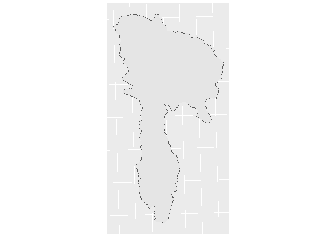
Figure 2.1: CS10 Basin, caclulated from the DEM.
The following code and commentary is from BuildR Script version 1.5.14, written by Christoph Schuerz.
BuildR recommends all layers to be in the same CRS, if we set project_layer to FALSE, it will throw an error when this is not the case:
The input layers might be in different coordinate reference systems (CRS). It is recommended to project all layers to the same CRS and check them before using them as model inputs. The model setup process checks if the layer CRSs differ from the one of the basin boundary. By setting ‘proj_layer <- TRUE’ the layer is projected if the CRS is different. If FALSE different CRS trigger an error.
We read in and check the basin boundary and run some checks
2.2.3 Processing the Land layer
Our land layer is located here:
Documentation on its creation does not exist.
lu_shp <- sf::read_sf(land_path)
lu_map <- ggplot2::ggplot(lu_shp) + ggplot2::geom_sf(ggplot2::aes(fill = type)) + sf_theme +
  ggplot2::theme(legend.position = "none")
print(lu_map)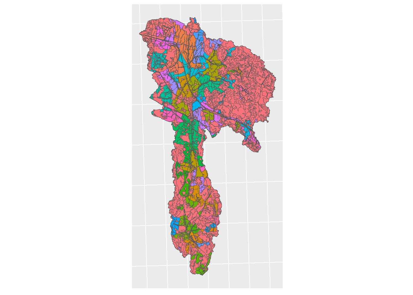
Figure 2.2: Land use map of CS10 by Farm ID
We had an issue with the classification of the land uses. For the OPTAIN project, all agricultural fields must have a unique ID, and our land uses only had the ID of the given farm KGB (which had many different fields). To remedy this, new IDs were generated with the format a_###f_# where a_ represents the farm, and f_ represents the respective field of that farm. The farm names needed to be shortened because the SWAT+ model often cannot handle long ID names (longer than 16 characters)
Note, the potential measures polygons were not counted as individual fields, which is why SP_ID does not match up with field_ID – This is by design.
## # A tibble: 6 × 4
##   KGB      type_fr sp_id field_ID
##   <chr>    <chr>   <dbl> <chr>
## 1 213/8/1  a_084       1 a_084f_1
## 2 213/7/6  a_083       2 a_083f_1
## 3 213/7/6  a_083       3 a_083f_2
## 4 213/7/4  a_082       4 a_082f_1
## 5 213/65/1 a_081       5 a_081f_1
## 6 213/65/1 a_081       6 a_081f_2
This was done in a simple QGIS workflow of dissolving by farm, splitting from single part to multipart, and then adding an iterating ID per farm field. This workflow could be replicated in R, and then shown here. It is under consideration…
BuildR will now run some checks on our land layer.
land <- read_sf(land_path) %>%
  check_layer_attributes(., type_to_lower = FALSE) %>%
  check_project_crs(layer = ., data_path =  data_path, proj_layer = project_layer,
                    label = 'land', type = 'vector')

check_polygon_topology(layer = land, data_path =  data_path, label = 'land',
                       area_fct =  0.00, cvrg_frc = 99.9,
                       checks = c(T,F,T,T,T,T,T,T))
BuildR splits the land layer into HRU (land) and reservoir (water) objects
2.2.4 Processing the Channels
No documentation exists on the creation of the channels layer, all we know is that it is located here:
channel_path <- 'model_data/input/line/cs10_channels_utm33n.shp'
channels <- read_sf(channel_path) %>% dplyr::select("type")
channel_map <- ggplot2::ggplot() + ggplot2::geom_sf(data = bound_sf) +
  ggplot2::geom_sf(data = channels, mapping = ggplot2::aes(color = type)) + sf_theme
channel_map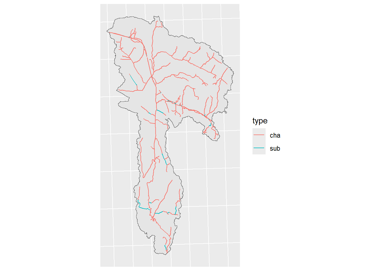
Figure 2.3: CS10 Channels including surface and subsurface channels
BuildR runs some checks:
 channel <- read_sf(channel_path) %>%
    check_layer_attributes(., type_to_lower = TRUE) %>%
    check_project_crs(layer = ., data_path =  data_path,
                      proj_layer = project_layer,
                      label = 'channel', type = 'vector')

check_line_topology(layer = channel, data_path = data_path,
                    label = 'channel', length_fct = 0, can_cross = FALSE)
BuildR then checks the connectivity between the channels and reservoirs. For this we need to define our id_cha_out and id_res_out.
“Variable id_cha_out sets the outlet point of the catchment. Either define a channel OR a reservoir as the final outlet. If channel then assign id_cha_out with the respective id from the channel layer. If reservoir then assign the respective id from the land layer to id_res_out, otherwise leave as NULL”
Running connectivity checks between channels and reservoirs:
Checking if any defined channel ids for drainage from land objects do not exist
2.2.5 Processing the DEM
BuildR loads and checks the DEM, and saves it.
dem <- rast(dem_path) %>%
  check_project_crs(layer = ., data_path =  data_path, proj_layer = project_layer,
                    label = 'dem', type = 'raster')
check_raster_coverage(rst = dem, vct_layer = 'land', data_path = data_path,
                      label = 'dem', cov_frc = 0.95)
save_dem_slope_raster(dem = dem, data_path = data_path)
Here is the result:
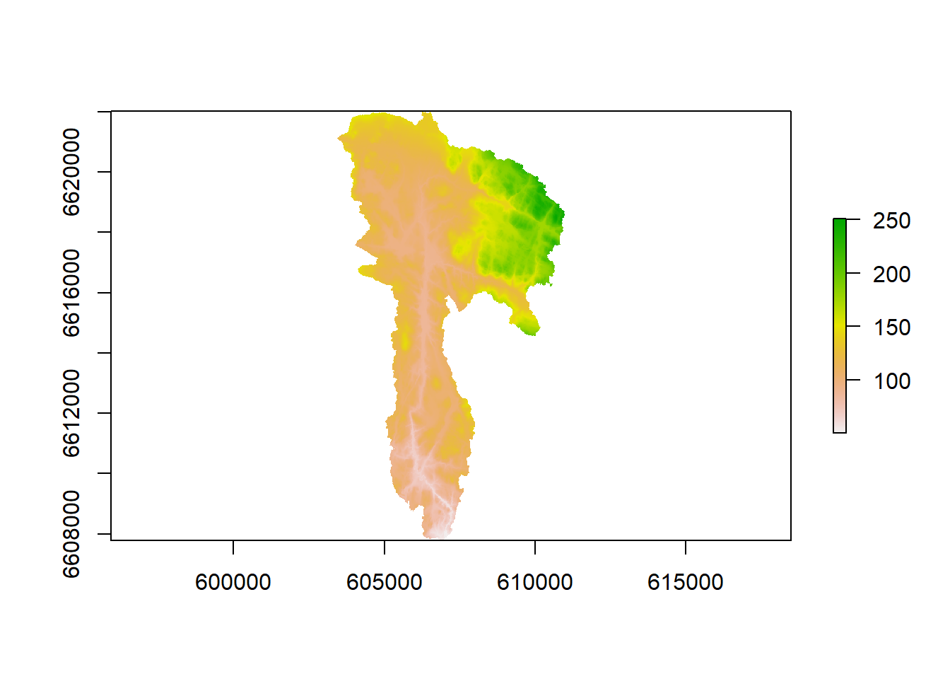
Figure 2.4: CS10 DEM cropped to basin
2.2.6 Processing Soil Data
Our soil map is located here:
No documentation exists on its creation.
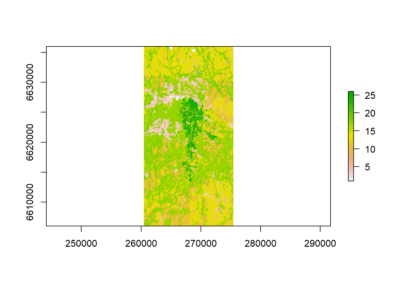
Figure 2.5: CS10 Soil map
The soil data and look-up path are located here:
soil_lookup_path <- 'model_data/input/soil/soil_lookup_26.csv'
soil_data_path   <- 'model_data/input/soil/usersoil_26_v2.csv'
Not much documentation exists here either. Some can be found in the excel sheet:
~/model_data/input/soil/swatsoil2.xlsx
BuildR reads in the soil data, performs checks, processes, and saves.
soil <- rast(soil_layer_path) %>%
  check_project_crs(layer = ., data_path =  data_path, proj_layer = project_layer,
                    label = 'soil', type = 'raster')
check_raster_coverage(rst = soil, vct_layer = 'hru', data_path = data_path,
                      label = 'soil', cov_frc = 0.75)
save_soil_raster(soil, data_path)
BuildR then generates a table with aggregated elevation, slope, soil for HRU units.
Read and prepare the soil input tables and a soil/hru id table and write them into data_path/tables.sqlite
2.3 Calculating Contiguous Object Connectivity
SWATBuildR follows COCOA. This section contains the calculations. You can read more about it in the protocol.
2.3.1 Calculating land unit connectivity
Preparing raster layers based on the DEM and the surface channel objects that will be used in the calculation of the land object connectivity.
The connection of each land object to neighboring land and water objects is calculated based on the flow accumulation and the D8 flow pointer along the object edge
2.3.1.1 Eliminate land object connections with small flow fractions:
For each land object the flow fractions are compared to connection with the largest flow fraction of that land object. Connections are removed if their fraction is smaller than frc_thres relative to the largest one.
This is necessary to:
Simplify the connectivity network
To reduce the risk of circuit routing between land objects. Circuit routing will be checked.
If an error due to circuit routing is triggered, then ‘frc_thres’ must be increased to remove connectivities that may cause this issue.
The remaining land object connections are analyzed for infinite loop routing. For each land unit the connections are propagated and checked if the end up again in the same unit.
# Analyzing land objects for infinite loop routing: Completed 6185 Land objects
# in 10M 44S
#
# ✘  150 Land objects identified where water is routed in loops.
#
# You can resolve this issue in the following ways:
#
#  - Use the layer 'land_infinite_loops.gpkg' that was written to
# model_data/cs10_setup/optain-cs10/data/vector to identify land polygons that
# cause the issue and split them to break the loops This would require to
# restart the entire model setup procedure!
#
#   - Increase the value of 'frc_thres'.
# This reduces the number of connections of each land unit (maybe undesired!)
# and can remove the connections that route the water in loops.
#
#   - Continue with the model setup (only recommended for small number of identified units!).
# The function 'resolve_loop_issues()' will then eliminate a certain number of
# connections.
What do we do here ? – I think in the past we just removed all the loops, but it says here it is not recommended when there are a lot of them. Should we increase the threshold? Should we try to break up the loops? You can see the problem polygons on the map below:
land_inifnite_loops_shp <- sf::read_sf("model_data/cs10_setup/optain-cs10/data/vector/land_infinite_loops.gpkg")
mapview::mapview(land_inifnite_loops_shp)
To me it seems to complicated to try to break up the loops, maybe increase the threshold a bit and see what happens? and delete the rest?
Increasing threshold and re-running leads to this:
frc_thres <- 0.1 #     loops (   mins)
frc_thres <- 0.2 # 238 loops (30 mins)
frc_thres <- 0.3 # 150 loops (12 mins)
frc_thres <- 0.4 # 115 loops (   mins)
frc_thres <- 0.5 # 94  loops (   mins)
frc_thres <- 0.6 # 57  loops (   mins)
We have decided that at a threshold of 0.3 and 150, we are within the “not that many” loops territory, considering out of 6000+ HRUs, it is only around 2%. Therefore we will let BuildR continue and remove them. This has been discussed in Issue #55.
2.4 Generate SWAT+ input
2.4.1 Generate land object SWAT+ input tables
Build the landuse.lum and a landuse/hru id table and write them into data_path/tables.sqlite
Build the HRU SWAT+ input files and write them into data_path/tables.sqlite
Add wetlands to the HRUs and build the wetland input files and write them into data_path/tables.sqlite
We only use the wetf land use .
2.4.2 Generate water object SWAT+ input tables
Build the SWAT+ cha input files and write them into data_path/tables.sqlite
Build the SWAT+ res input files and write them into data_path/tables.sqlite
Build SWAT+ routing unit con_out based on ‘land_connect_fraction’.
Build the SWAT+ rout_unit input files and write them into data_path/tables.sqlite
Build the SWAT+ LSU input files and write them into data_path/tables.sqlite
2.4.3 Build aquifer input
Build the SWAT+ aquifer input files for a single aquifer for the entire catchment. The connectivity to the channels with geomorphic flow must be added after writing the txt input files. This is not implemented in the script yet.
2.4.4 Add point source inputs
Point sources have been prepared in Section REF
The point source locations are provided with a point vector layer in the path ‘point_path’.
Maximum distance of a point source to a channel or a reservoir to be included as a point source object (recall) in the model setup:
Adding the point sources with BuildR: